Machine-translated from Chinese.
局部标准型
我们知道研究曲线局部性质的时候, 利用Frenet标架来处理会方便很多.
取(无一阶奇点) 弧长参数化曲线$\alpha:I\rightarrow \mathbb{R}^3,$
由Taylor展开,
$\alpha(s)=\alpha(0)+s\alpha'(0)+\frac{s^2}{2}\alpha''(0)+\frac{s^3}{6}\alpha'''(0)+R,$
$R=o(s^3).$ 我们知道$\alpha'(0)=t,$ $\alpha''(0)=kn,$
$\alpha'''(0)=(kn)'=k'n+kn'=k'n-k^2t-k\tau b.$
整理得到$\alpha(s)-\alpha(0)=(s-\frac{k^2s^3}{6})t+(\frac{s^2k}{2}+\frac{s^3k'}{6})n-\frac{s^3}{6}k\tau b+R,$
从而我们便得到在Frenet标架下曲线的(高阶)局部近似坐标:
$$\left\{
\begin{aligned}
x(s)&=s-\frac{k^2s^3}{6}+R_x\\
y(s)&=\frac{k}{2}s^2+\frac{k's^3}{6}+R_y\\
z(s)&=-\frac{k\tau}{6}s^3+R_z
\end{aligned}
\right.$$
上式称为曲线$\alpha$在零点邻域的局部标准型. 用一阶视角来看,
只能看到切向量$t,$ 即只有$x$方向上的信息; 而用三阶视角来看,
就能看到在$\mathbb{R}^3$中的更多信息, 比如曲线的转向($n$方向),
爬升($b$方向)等等.
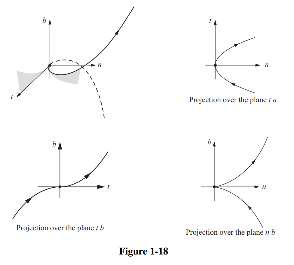
由此看出一些几何性质: 当挠率为负时,
局部来看曲线是上穿密切平面(osculating)的; 而正挠率的曲线是下穿的.
从切平面(rectifying)可以在某邻域内将曲线划分在一侧$(k\neq 0).$
关于密切平面的一个重要信息是, 它是距离曲线最近(最致密)的一个平面.
用数学语言说明即,
它是$s$点处切线和$s+h$点决定的平面在$h\rightarrow 0$时的极限.
不妨设$s=0,$ 由Frenet标架与局部标准型,
可记该平面为$z=cy$(从切平面$y=0$排除).
那么计算$c=\frac{z(h)}{y(h)}=\frac{-\frac{k\tau}{6}h^3+o(h^3)}{\frac{k}{2}h^2+o(h^2)}=-\frac{\tau h}{3}+o(h).$
从而平面趋于$z=0,$ 即密切平面.
注记 1.1. 有的书中可能会将挠率定义为$b'=-\tau n,$ 需要注意.
来做几道练习. 我们提到从切平面可以在$P$点某邻域内将曲线划分在一侧,
事实上任意含$P$点切线的平面, 除了密切平面都可以.
只需考察将曲线沿$x$轴(切方向)投影在法平面,
那么前面的$z=cy$即为该曲线零点和$h$点的割线, 割线的斜率趋于零.
所以对于任意给定的平面$z=c_0y,$ $c_0\neq 0,$
总能找到足够小的邻域使得割线斜率小于$c_0,$
从而投影曲线保持在$z=c_0 y$直线下方, 也就是原曲线保持在平面一侧.
密切平面也可以由其他的方式确定,
比如$\alpha(s),\alpha(s+h_1),\alpha(s+h_2)$三点所确定的平面在$h_1,h_2\rightarrow 0$时的极限.
同样取局部标准型, 那么平面可记为$ax+by+cz=0.$
取$F(s)=ax(s)+by(s)+cz(s),$ 那么$F'(0)=a,$ $F''(0)=bk.$
这里$a,b$为关于$h_1,h_2$的函数. 由于$F(0),F(h_1),F(h_2)=0,$
由中值定理即知$a,b\rightarrow 0.$ 从而平面趋于$z=0,$ 即密切平面.
一个经典的结论是曲线在$P$点的曲率与投影在$P$点密切平面曲线在该点的曲率是一致的.
这是因为由局部标准型,
$P$点$(s=0)$曲率可由$\lim\limits_{s\rightarrow 0}\frac{2y(s)}{x^2(s)}$决定,
与$z$无关.
平面曲线整体性质
接下来讨论一些平面曲线的整体微分性质. 第五章会更系统地讨论,
感兴趣的同学可以之后看一下.
做一些简单的回顾,
平面闭曲线$\alpha:[a,b]\rightarrow R^2$在要求$\alpha(a)=\alpha(b)$的同时,
还要求高阶导数一致. 它是简单的, 如果该闭曲线不自交.
一般也是做弧长参数化的, 同时平面曲线的曲率会出现正负号.
我们说平面内的简单闭曲线会框住一个内部区域, 这可由Jordan曲线定理得到,
参见第五章. 若沿曲线参数增加的方向看, 内部始终保持在曲线左侧,
则称曲线是正定向的.
等周不等式
这是微分几何中最古老的整体问题. 等长的简单闭曲线何时围住最大面积?
Weierstrass最早给出了变分方法的证明, 但比较繁琐.
这里介绍Schmidt于1939年给出的证明. 对于曲线所围的区域, 由Green公式,
我们有面积计算公式:
$$A=-\int_{a}^b yx'dt=\int_a^bxy'dt=\frac{1}{2}\int_a^b xy'-yx'dt.$$
或者如书中通过初等方法来证明, 但方法实质类似Green公式的初等证明,
且需要承认一些结论(能够找到一条直线,
使得曲线关于该直线的距离函数有有限多个极值点).
定理 1.2 (等周不等式). 设$C$为长度为$l$的平面简单闭曲线, $A$为$C$所围面积, 则$l^2-4\pi A\ge 0,$ 等号成立当且仅当$C$为圆周.
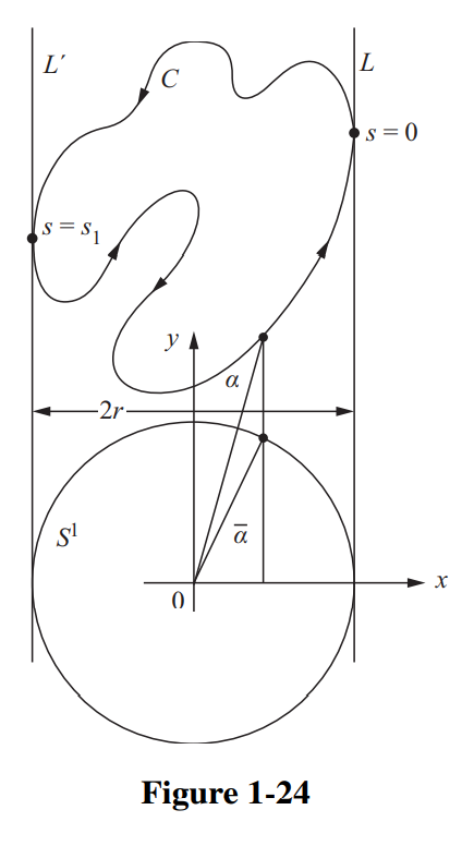
证: 如图所示, 取合适的平行线$L,L'$卡住曲线$C$.
在下方取一个半径为$r$同样被卡住的圆$S^1$, 以圆心为原点,
垂直$L,L'$方向为$x$轴, 沿$L,L'$方向为$y$轴建系.
对$C$做弧长参数化$\alpha(s)=(x(s),y(s)).$
设$S^1$曲线为$\bar\alpha(s)=(x(s),\bar y(s)),$ 即$x$方向两曲线同步.
由面积公式, 我们有: $$\begin{aligned}
A+\pi r^2=\int_0^l(xy'-\bar yx')ds\le \int_0^l\sqrt{x^2+\bar y^2} \cdot \sqrt{ {y'}^2+{x'}^2}ds=lr.
\end{aligned}$$
从而由几何平均值$\sqrt{A}\sqrt{\pi r^2}\le \frac{1}{2}(A+\pi r^2)\le \frac{1}{2}lr,$
$4 \pi A r^2\le l^2 r^2,$ 即$l^2-4\pi A\ge 0.$ (注意与$r$无关.)
当等号成立时, 所有不等式取等. 由几何平均不等式, $A=\pi r^2.$
从而$l=2\pi r,$ 且任意旋转$L,L'$方向, 间距仍为$2r$.
同时$(x,\bar y)=\lambda (y',-x'),$ 由模长关系知$|\lambda|=r,$
从而$x=\pm r y'.$ 将$L,L'$旋转$90$度, 又得到$y=\pm r x'.$
于是$x^2+y^2=r^2({x'}^2+{y'}^2)=r^2,$ 即$C$为圆周.
注记 1.3. 易见等周不等式对$C^1$简单闭曲线即成立, 对分段$C^1$的也自然成立. (未加说明时, 默认光滑.)
四顶点定理
对弧长参数化后的闭曲线$\alpha(s)=(x(s),y(s)),$
引入切线标线$t(s)=(x'(s),y'(s)).$ 其轨迹落在单位圆周上,
且速度向量为$kn$. 记$\theta(s)$为$t(s)$与$x$轴交角,
若限制其落在$[0,2\pi)$上, 则$\theta$不见得连续.
由于其可局部用反三角函数定义$(\theta(s)=\arctan\frac{y'(s)}{x'(s)}(+\pi)),$
它是可微的.
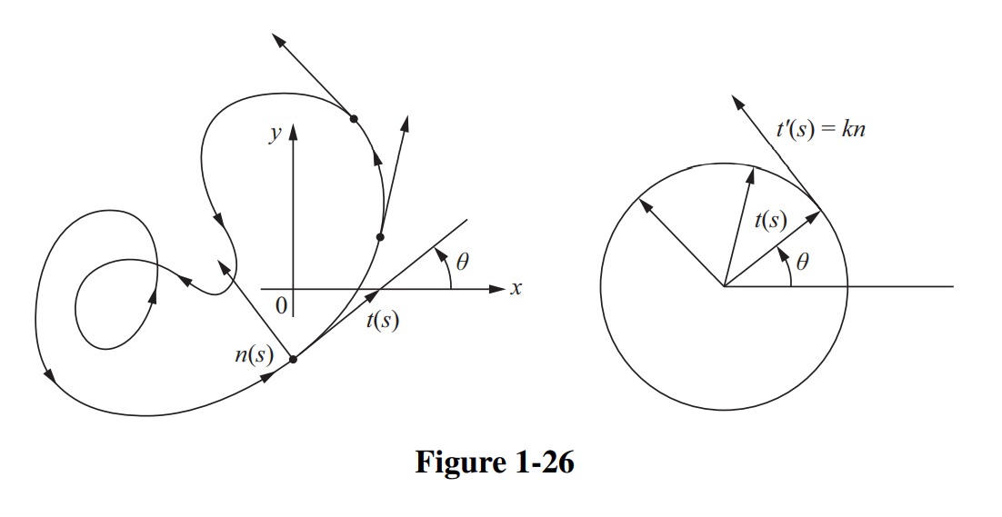
由$t(s)=(\cos \theta(s),\sin \theta(s)),$ 速度向量$t'=\theta' n,$
即$\theta'=k.$
从而可以整体地重新定义连续函数$\theta(s)=\int_0^s k(s)ds.$
它与原先的函数相差$2k\pi.$ 该函数描述了切向量的总旋转角度,
由于闭曲线始末切向量相同, 旋转角度是$2\pi$的整数倍.
记$\int_0^l k(s)ds=\theta(l)-\theta(0)=2\pi I,$
称整数$I$为曲线$\alpha$的旋转指标. 注意由于$k$是带符号的,
旋转指标$I$也是. 当简单闭曲线正定向时, 旋转指标也是正的.
我们有如下定理, 于5.7节定理2中给出证明:
定理 1.4 (旋转指标定理). 简单闭曲线的旋转指标为$\pm 1,$ 正负号取决于曲线的定向.
接下来引入曲线顶点的概念.
称正则平面曲线$\alpha:[a,b]\rightarrow \mathbb{R}^2$是凸的,
若$\,\forall\,t\in [a,b],$ $\alpha$的轨迹始终落在$t$点切线一侧.
而平面曲线的顶点, 定义为使得$k'(t)=0$的全体点$t$,
即曲率的全体驻点(部分书中会更精确地定义为极值点). 举例来说,
椭圆恰有四个顶点. 有趣的是, 任意简单凸的闭曲线都至少有四个顶点.
首先证明一个引理.
引理 1.5. 记$\alpha(s)=(x(s),y(s)):[0,l]\rightarrow \mathbb{R}^2$为弧长参数化平面闭曲线. 则$\,\forall\,A,B,C\in \mathbb{R},$ $\int_0^l(Ax+By+C)k'ds=0.$
证: 由开头定义的$\theta$函数,
我们有$(x',y')=(\cos \theta,\sin \theta),$ $k=\theta'$且$x''=-ky',$
$y''=kx'.$ 从而对于闭曲线, 有$\int_0^l k'ds=0,$
$\int_0^l xk'ds=-\int_0^lkx'ds=-\int_0^ly''ds=0,$
$\int_0^l yk'ds=-\int_0^lky'ds=\int_0^lx''ds=0.$ 从而引理得证.
定理 1.6 (四顶点定理). 简单凸的闭曲线至少有四个顶点.
证: 将曲线弧长参数化, 只需考察$[0,l]$上连续函数$k(s)$的行为.
由于其为周期函数, 最大值点和最小值点都是驻点.
因此我们已经找到了两个顶点$p,q.$ 这两点划分出两端弧, 过$p,q$作直线$L$,
首先需要说明每段弧保持在$L$的一侧.
不然, 假设某段弧还与$L$相交于点$r$, 那么对于$L$上三点$p,q,r$,
选取中间的点不妨为$p$. $p$点切线必须恰为$L$, 不然$q,r$在切线两侧,
与凸性矛盾. 然而即使$p$点切线为$L$,
$p$点附近的切线也仍会将$q,r$划分在切线两侧, 与凸性矛盾,
除非$p$点附近保持为直线, 到$q,r$为止. 这时在$p,q$最值点处$k=0$,
这说明$k\equiv 0$, 不可能为闭曲线.
另一方面, 若两端弧保持在$L$的同一侧, 则由凸性类似可得某段弧退化为直线,
同理矛盾. 因此两端弧在$L$的两侧. 记$Ax+By+C=0$为直线$L$的方程.
如果不再有其它顶点, 那么$k'$在两段弧上分别恒负, 恒正.
进而可调整符号使得$C$上除$p,q$点外$(Ax+By+C)k'$恒正. 这与前面的引理矛盾,
从而可以找到第三个顶点位于某段弧上, 且在该点$k'$改变符号.
由于弧连接了$k(s)$的最小值点和最大值点, $k'(s)$符号改变偶数次,
因此在这段弧上必能找到第四个顶点.
四顶点定理一直是许多研究的课题, 事实上该定理对简单闭曲线即成立,
但证明要复杂一些, 可查看参考文献. 前面一直提到简单凸的闭曲线,
但事实上有些多余. 5.7节命题1将证明平面闭曲线是凸的当且仅当它是简单的,
且存在定向使得曲率非负. 因此可以如下更精确地表述四顶点定理:
定理 1.7 (四顶点定理’). 存在定向使得闭凸曲线曲率函数非负, 且(严格)极大值点和极小值点分别至少有两个, 或曲率恒为常数(此时曲线即为圆周).
一个自然的问题是, 对于任意给定的周期函数$k:[a,b]\rightarrow \mathbb{R},$
若其满足四顶点定理的结论,
是否能够找到一个简单闭曲线使得$k$成为其曲率函数?
也就是四顶点定理的逆命题. 这类似于三维空间中的曲线论基本定理.
对于函数严格正的情况, H.Gluck于1971年给出了肯定的答案.
B.Dahlberg于1997年得到了完整的逆定理.
四顶点定理及其逆定理这一专题于2005经过编辑与整合发表了一篇非常详尽的论文,
感兴趣的同学可以查看一下.
Cauchy-Crofton公式
我们先直接给出这一有趣的定理, 后面只给出定理的证明思路:
定理 1.8 (Cauchy-Crofton公式). 令$C$为长度为$l$的平面正则曲线, 则所有与$C$有交点的(带重数的)直线全体测度为$2l.$
这里需要说明两点, 首先重数指直线与曲线$C$的交点个数,
即若某直线与曲线$C$有$n$个交点, 那么该直线在集合中记$n$次.
其次需要说明测度是什么.
取垂直于直线的单位向量$v=(\cos \theta,\sin \theta)$,
记$p$为直线上任一点与$v$的内积, 那么直线完全由这两个参数决定.
记直线全体为$\mathcal{L}=\{(p,\theta)\in \mathbb{R}^2; (p,\theta)\sim (-p,\theta+\pi)\},$
我们说明其上可以唯一定义合理的测度.
这里合理即指我们希望测度在刚性变换下保持不变. 首先有如下简单的命题:
命题 1.9. 记$f(x,y)$为$\mathbb{R}^2$上连续函数, 对集合$S\subset \mathbb{R}^2,$ 定义其面积$A(S)=\iint_S f(x,y)dxdy.$ 若$A$为刚性变换不变量, 则$f$必为常数.
证: 记刚性变换为$F$. 由于刚性变换Jacobian为$1$,
我们有$A(F(S))=\iint_S f(F(x,y))dxdy=\iint_S f(x,y)dxdy=A(S).$
由于对任意$S$成立, $f\circ F=f.$ 又由刚性变换在$\mathbb{R}^2$是可迁的,
即$\,\forall\,p,q\in \mathbb{R}^2,$
$\,\exists\,$刚性变换$F$使得$F(p)=q,$ 即知$f=\text{const}.$
对于$\mathcal{L}$中曲线$x\cos\theta+y\sin\theta=p,$
其在刚性变换$\begin{cases}
\bar x=a+x\cos \varphi -y\sin \varphi\\
\bar y=b+x\sin \varphi +y\cos \varphi
\end{cases}$下, 参数变为$\begin{cases}
\bar \theta=\theta + \varphi\\
\bar p=p+a\cos(\theta+\varphi)+b\sin(\theta+\varphi)
\end{cases}.$ 易见该变换在$(p,\theta)$坐标下Jacobian也为$1,$
同时该作用在直线全体$\mathcal{L}$上显然是可迁的,
因此同理可知测度可相差常数倍地唯一定义为$\mu(\mathcal{G})=\iint_\mathcal{G} dpd\theta$,
这一测度被称为kinematic(运动学上的)测度.
接下来我们给出定理证明的大体思路.
证: 对于$l$长的直线段$C,$ 由于测度在刚性变换下不变,
不妨设$C$以原点为中心, 落在$x$轴上. 那么所求集合的测度为:
$$\int_0^{2\pi} \int_0^{|\cos\theta|l/2}dpd\theta=\int_0^{2\pi}\frac{l}{2}|\cos\theta |d\theta=2l.$$
接下来, 对于由有限多个线段拼成的折线$C,$ 将每个线段对应的直线的测度做和,
即可得到带重数的所求集合的测度为$\iint n(p,\theta)dpd\theta=2\sum_i l_i=2l.$
最后取极限, 我们可以期望如上公式对任意正则曲线均适用, 这就证明了定理.
需要注意的一点是, 对于直线段, 其实会出现重数为无穷的直线,
但它在kinematic测度下零测. 对于书上的证明,
将取极限的过程精确描述较为繁琐. 一个更为具体的证明如下:
证: 对$(p,\theta)$对应的直线,
也可将其转为更常见的先确定点$Z(s)=(x(s),y(s))\in C,$ 再确定角度$\eta.$
即将$(p,\theta)$坐标转换为$(s,\eta)$坐标. 这里令$\theta=\eta,$
几何意义相同. 那么$p=x(s)\cos \eta+y(s)\sin \eta.$
注意到$(x',y')$可表示为$(\cos\phi,\sin \phi),$
那么Jacobian为$|\cos(\phi(s)-\eta)|.$
从而由Fubini定理, 所求测度为: $$\begin{aligned}
\int_{\left\{L:L\cap C\neq \varnothing\right\} }ndpd\theta&=\int_{\left\{L:L\cap C\neq \varnothing\right\} }(\sum_{Z\in L\cap C}1)dpd\theta\\
&=\int_{\left\{Z:Z\in C\right\} }\int_{\left\{L:Z\in L\right\} }dpd\theta\\
&=\int_0^{l}\int_{0}^{\pi} |\cos(\phi(s)-\eta)|d\eta ds\\
&=\int_0^l 2 ds=2l.
\end{aligned}$$
这一主题的基本思想归于Integral Geometry这一分支.
一个Cauchy-Crofton公式的有趣应用是用来估计曲线长度.
取一族等间距$r$的直线, 再等角度地$\alpha$地旋转扫过整个平面,
则$l=\frac{1}{2}\int ndpd\theta\approx \frac{1}{2}nr\alpha,$
$n$为曲线与这些直线的总交点数(记重数), 即将积分离散化.
书中提到这在生物学等领域中有所应用, 如估计DNA分子长度.
文章最后更新于 2021-08-11 12:07:07
Local Normal Form
We know that when studying the local properties of curves, it is much more convenient to use the Frenet frame.
Take (no first-order singularity) arc length parameterized curve $\alpha:I\rightarrow \mathbb{R}^3,$
Expanded by Taylor,
$\alpha(s)=\alpha(0)+s\alpha'(0)+\frac{s^2}{2}\alpha''(0)+\frac{s^3}{6}\alpha'''(0)+R,$
$R=o(s^3).$ We know $\alpha'(0)=t,$ $\alpha''(0)=kn,$
$\alpha'''(0)=(kn)'=k'n+kn'=k'n-k^2t-k\tau b.$
Organize to get $\alpha(s)-\alpha(0)=(s-\frac{k^2s^3}{6})t+(\frac{s^2k}{2}+\frac{s^3k'}{6})n-\frac{s^3}{6}k\tau b+R,$
Thus we obtain the (higher-order) local approximate coordinates of the curve under the Frenet frame:
$$\left\{
\begin{aligned}
x(s)&=s-\frac{k^2s^3}{6}+R_x\\
y(s)&=\frac{k}{2}s^2+\frac{k's^3}{6}+R_y\\
z(s)&=-\frac{k\tau}{6}s^3+R_z
\end{aligned}
\right.$$
The above formula is called the local standard form of the curve $\alpha$ in the zero point neighborhood. Viewed from a first-order perspective,
Only the tangent vector $t,$ can be seen, that is, only the information in the $x$ direction; and from a third-order perspective,
You can see more information in $\mathbb{R}^3$, such as the direction of the curve ($n$ direction),
Climb ($b$ direction) etc.
From this we can see some geometric properties: When the torsion is negative,
Locally, the curve goes up through the osculating plane; while the curve with positive torsion goes down.
From the tangent plane (rectifying), the curve can be divided on one side in a certain neighborhood $(k\neq 0).$
An important piece of information about the oblique plane is that it is the closest (most dense) plane to the curve.
In mathematical language, that is,
It is the limit of the plane determined by the tangent at point $s$ and point $s+h$ at $h\rightarrow 0$.
Let's suppose that $s=0,$ consists of Frenet frame and local standard form,
This plane can be recorded as $z=cy$ (excluded from the tangent plane $y=0$).
Then calculate $c=\frac{z(h)}{y(h)}=\frac{-\frac{k\tau}{6}h^3+o(h^3)}{\frac{k}{2}h^2+o(h^2)}=-\frac{\tau h}{3}+o(h).$
Therefore, the plane tends to $z=0,$, which is the close plane.
Note 1.1. Some books may define torsion as $b'=-\tau n,$. Please note.
Let’s do some exercises. We mentioned that from the tangent plane, the curve can be divided on one side in a certain neighborhood of the $P$ point,
In fact, any plane containing the tangent line of point $P$ can be used, except the close plane.
Just consider the projection of the curve along the $x$ axis (tangential direction) on the normal plane,
Then the previous $z=cy$ is the secant line between the zero point of the curve and the $h$ point, and the slope of the secant line tends to zero.
So for any given plane $z=c_0y,$ $c_0\neq 0,$
It is always possible to find a small enough neighborhood such that the secant slope is less than $c_0,$
Therefore, the projected curve remains below the $z=c_0 y$ line, that is, the original curve remains on the plane side.
The close plane can also be determined in other ways,
For example, the limit of the plane determined by the three points $\alpha(s),\alpha(s+h_1),\alpha(s+h_2)$ is at $h_1,h_2\rightarrow 0$.
Also take the local standard form, then the plane can be recorded as $ax+by+cz=0.$
Take $F(s)=ax(s)+by(s)+cz(s),$ then $F'(0)=a,$ $F''(0)=bk.$
Here $a,b$ is a function about $h_1,h_2$. Since $F(0),F(h_1),F(h_2)=0,$
From the mean value theorem, we know that $a,b\rightarrow 0.$ and the plane tend to $z=0,$, that is, the close plane.
A classic conclusion is that the curvature of the curve at point $P$ is consistent with the curvature of the close plane curve projected at point $P$ at that point.
This is because from the local standard type,
The curvature of $P$ point $(s=0)$ can be determined by $\lim\limits_{s\rightarrow 0}\frac{2y(s)}{x^2(s)}$,
Has nothing to do with $z$.
Overall properties of plane curves
Next, we discuss the global differential properties of some plane curves. Chapter 5 will discuss them more systematically,
Interested students can take a look later.
Do some simple review,
Plane closed curve $\alpha:[a,b]\rightarrow R^2$ requires $\alpha(a)=\alpha(b)$ at the same time,
It is also required that the higher order derivatives are consistent. It is simple , if the closed curve does not self-intersect.
Generally, the arc length is parameterized, and the curvature of the plane curve will have positive and negative signs.
We say that a simple closed curve in the plane will frame an internal region, which can be obtained from the Jordan Curve Theorem,
See Chapter 5. If you look in the direction in which the curve parameters increase, the interior always remains on the left side of the curve.
Then the curve is said to be Positive orientation of.
equal period inequality
This is the oldest overall problem in differential geometry. When do simple closed curves of equal length enclose the largest area?
Weierstrass gave the earliest proof of the variational method, but it was rather cumbersome.
Here we introduce the proof given by Schmidt in 1939. For the area enclosed by the curve, according to Green's formula,
We have the formula for calculating area:
$$A=-\int_{a}^b yx'dt=\int_a^bxy'dt=\frac{1}{2}\int_a^b xy'-yx'dt.$$
Or as the book proves through elementary methods, but the method is essentially similar to the elementary proof of Green's formula,
And need to admit some conclusions (can find a straight line,
Such that the distance function of the curve with respect to the straight line has a finite number of extreme points).
Theorem 1.2 (Equal period inequality). Assume $C$ is a plane simple closed curve with length $l$, $A$ is the area enclosed by $C$, then $l^2-4\pi A\ge 0,$ is equal if and only if $C$ is the circumference.
Certificate: As shown in the figure, take a suitable parallel line $L,L'$ and clamp the curve $C$.
Take a circle $S^1$ with a radius $r$ below that is also stuck, with the center of the circle as the origin,
The vertical $L,L'$ direction is the $x$ axis, and the $L,L'$ direction is the $y$ axis.
Parameterize arc length $\alpha(s)=(x(s),y(s)).$ for $C$
Assume the $S^1$ curve is $\bar\alpha(s)=(x(s),\bar y(s)),$, that is, the two curves in the $x$ direction are synchronized.
From the area formula, we have: $$\begin{aligned}
A+\pi r^2=\int_0^l(xy'-\bar yx')ds\le \int_0^l\sqrt{x^2+\bar y^2} \cdot \sqrt{ {y'}^2+{x'}^2}ds=lr.
\end{aligned}$$
Thus by the geometric mean $\sqrt{A}\sqrt{\pi r^2}\le \frac{1}{2}(A+\pi r^2)\le \frac{1}{2}lr,$
$4 \pi A r^2\le l^2 r^2,$ is $l^2-4\pi A\ge 0.$ (note that it has nothing to do with $r$.)
When the equal sign holds, all inequalities are equal. From the geometric mean inequality, $A=\pi r^2.$
Therefore, $l=2\pi r,$ and any rotation $L,L'$ direction, the distance is still $2r$.
At the same time $(x,\bar y)=\lambda (y',-x'),$ it is known from the module length relationship $|\lambda|=r,$
Thus $x=\pm r y'.$ rotates $L,L'$ by $90$ degrees, and gets $y=\pm r x'.$
So $x^2+y^2=r^2({x'}^2+{y'}^2)=r^2,$ or $C$ is the circumference of the circle.
Note 1.3. It is easy to see that the equal period inequality is established for the simple closed curve $C^1$, and it is also naturally established for the segmented $C^1$. (When not specified, the default is smooth.)
four vertex theorem
Closed curve parameterized for arc length $\alpha(s)=(x(s),y(s)),$
Introduce the tangent mark $t(s)=(x'(s),y'(s)).$ whose trajectory falls on the unit circle,
And the speed vector is $kn$. Let $\theta(s)$ be the intersection angle between the $t(s)$ and $x$ axes,
If it is restricted to fall on $[0,2\pi)$, $\theta$ may not be continuous.
Because it can be defined locally by inverse trigonometric functions $(\theta(s)=\arctan\frac{y'(s)}{x'(s)}(+\pi)),$
It is differentiable.
From $t(s)=(\cos \theta(s),\sin \theta(s)),$ velocity vector $t'=\theta' n,$
That is $\theta'=k.$
Thus continuous functions can be redefined as a whole $\theta(s)=\int_0^s k(s)ds.$
It differs from the original function $2k\pi.$. This function describes the total rotation angle of the tangent vector,
Since the tangent vectors at the beginning and end of the closed curve are the same, the rotation angle is an integer multiple of $2\pi$.
Note$\int_0^l k(s)ds=\theta(l)-\theta(0)=2\pi I,$
Call the integer $I$ the curve $\alpha$ Rotation indicator. Note that since $k$ is signed,
The same goes for the rotation indicator $I$. When the simple closed curve has a positive orientation, the rotation indicator is also positive.
We have the following theorem, which is proved in Theorem 2 of Section 5.7:
Theorem 1.4 (Rotation Index Theorem). The rotation index for a simple closed curve is $\pm 1,$ whose sign depends on the orientation of the curve.
Next, the concept of curve vertices is introduced.
The regular plane curve $\alpha:[a,b]\rightarrow \mathbb{R}^2$ is said to be convex of,
If the trajectory of $\,\forall\,t\in [a,b],$ $\alpha$ always falls on the tangent side of point $t$.
And the plane curve vertex, defined as all points $t$ such that $k'(t)=0$,
That is, the global stationary point of curvature (some books will define it more accurately as an extreme point). For example,
An ellipse has exactly four vertices. Interestingly, any simple convex closed curve has at least four vertices.
First prove a lemma.
Lemma 1.5. Let $\alpha(s)=(x(s),y(s)):[0,l]\rightarrow \mathbb{R}^2$ be the arc length parameterized plane closed curve. Then $\,\forall\,A,B,C\in \mathbb{R},$ $\int_0^l(Ax+By+C)k'ds=0.$
Certificate: The $\theta$ function defined at the beginning,
We have $(x',y')=(\cos \theta,\sin \theta),$ $k=\theta'$ and $x''=-ky',$
$y''=kx'.$ Thus for a closed curve, there is $\int_0^l k'ds=0,$
$\int_0^l xk'ds=-\int_0^lkx'ds=-\int_0^ly''ds=0,$
$\int_0^l yk'ds=-\int_0^lky'ds=\int_0^lx''ds=0.$ Thus the lemma is proved.
Theorem 1.6 (Four Vertices Theorem). A simple convex closed curve has at least four vertices.
Certificate: To parameterize the arc length of the curve, we only need to examine the behavior of the continuous function $k(s)$ on $[0,l]$.
Since it is a periodic function, the maximum value point and the minimum value point are both stationary points.
Therefore, we have found two vertices $p,q.$. These two points divide the arcs at both ends, and draw a straight line $L$ through $p,q$,
First, it needs to be stated that each arc remains on one side of $L$.
Otherwise, assuming that a certain arc also intersects $L$ at point $r$, then for the three points $p,q,r$ above $L$,
Select the middle point as $p$. The tangent line at $p$ point must be exactly $L$, otherwise $q,r$ will be on both sides of the tangent line.
Contradictory to convexity. However, even if the tangent line of point $p$ is $L$,
The tangent line near point $p$ will still divide $q,r$ on both sides of the tangent line, which is inconsistent with convexity.
Unless the straight line remains near point $p$ until $q,r$. At this time, at $k=0$, the maximum point of $p,q$,
This shows that $k\equiv 0$ cannot be a closed curve.
On the other hand, if the two end arcs remain on the same side of $L$, then a certain arc can be degenerated into a straight line due to the similarity of convexity,
The same contradiction occurs. Therefore, the two end arcs are on both sides of $L$. Let $Ax+By+C=0$ be the equation of the straight line $L$.
If there are no other vertices, then $k'$ is always negative and always positive on the two arcs.
Furthermore, the sign can be adjusted so that $(Ax+By+C)k'$ on $C$ is always positive except for the point $p,q$. This is contradictory to the previous lemma,
Thus, it can be found that the third vertex is located on a certain arc, and the sign changes at this point $k'$.
Since the arc connects the minimum and maximum points of $k(s)$, the sign of $k'(s)$ changes an even number of times,
Therefore, the fourth vertex must be found on this arc.
The four-vertex theorem has been the subject of many studies. In fact, the theorem is true for simple closed curves.
But the proof is a little more complicated, you can check the references. As mentioned before simple convex closed curve,
But in fact it is somewhat redundant. Proposition 1 of Section 5.7 will prove that a plane closed curve is convex if and only if it is simple,
And there is an orientation such that the curvature is non-negative. Therefore, the four-vertex theorem can be expressed more accurately as follows:
Theorem 1.7 (Four Vertices Theorem’). There is an orientation such that the curvature function of the closed convex curve is non-negative, and there are at least two (strictly) maximum points and minimum points, or the curvature is constant (in this case, the curve is a circle).
A natural question is, for any given periodic function $k:[a,b]\rightarrow \mathbb{R},$
If it satisfies the conclusion of the four vertex theorem,
Is it possible to find a simple closed curve such that $k$ becomes its curvature function?
That is the converse proposition of the four-vertex theorem. This is similar to the fundamental theorem of curve theory in three-dimensional space.
For the case where the function is strictly positive, H.Gluck gave an affirmative answer in 1971.
B.Dahlberg obtained the complete inverse theorem in 1997.
The topic of the four-vertex theorem and its inverse theorem was edited and integrated into a very detailed paper in 2005.
Interested students can check it out.
Cauchy-Crofton formula
We first give this interesting theorem directly, and then only give the proof of the theorem:
Theorem 1.8 (Cauchy-Crofton formula). Let $C$ be a plane regular curve with length $l$, then the overall measure of all straight lines (with multiplicity) that have intersection points with $C$ is $2l.$
Two points need to be explained here. First, the multiplicity refers to the number of intersection points between the straight line and the curve $C$.
That is, if a straight line has $n$ intersection points with the curve $C$, then the straight line is recorded $n$ times in the set.
Secondly, we need to explain what the measure is.
Take the unit vector $v=(\cos \theta,\sin \theta)$ perpendicular to the straight line,
Let $p$ be the inner product of any point on the straight line and $v$, then the straight line is completely determined by these two parameters.
Record the entire straight line as $\mathcal{L}=\{(p,\theta)\in \mathbb{R}^2; (p,\theta)\sim (-p,\theta+\pi)\},$
We show that a reasonable measure can be uniquely defined on it.
Reasonable here means that we hope that the measure remains unchanged under rigid transformation. First, there is the following simple proposition:
Proposition 1.9. Let $f(x,y)$ be a continuous function on $\mathbb{R}^2$, and define its area $A(S)=\iint_S f(x,y)dxdy.$ for the set $S\subset \mathbb{R}^2,$. If $A$ is a rigid transformation invariant, then $f$ must be a constant.
Certificate: Let the rigid transformation be $F$. Since the Jacobian rigid transformation is $1$,
We have $A(F(S))=\iint_S f(F(x,y))dxdy=\iint_S f(x,y)dxdy=A(S).$
Since it is true for any $S$, $f\circ F=f.$ is transitive to $\mathbb{R}^2$ due to rigid transformation,
That is $\,\forall\,p,q\in \mathbb{R}^2,$
$\,\exists\,$ Rigid transformation $F$ makes $F(p)=q,$ known $f=\text{const}.$
For curve $x\cos\theta+y\sin\theta=p,$ in $\mathcal{L}$
Under the rigid transformation $\begin{cases}
\bar x=a+x\cos \varphi -y\sin \varphi\\
\bar y=b+x\sin \varphi +y\cos \varphi
\end{cases}$, the parameter becomes $\begin{cases}
\bar \theta=\theta + \varphi\\
\bar p=p+a\cos(\theta+\varphi)+b\sin(\theta+\varphi)
\end{cases}.$. It is easy to see that the Jacobian of this transformation under the $(p,\theta)$ coordinate is also $1,$.
At the same time, this effect is obviously transitive on the entire straight line $\mathcal{L}$.
Therefore, in the same way, it can be seen that the measure can be uniquely defined as $\mu(\mathcal{G})=\iint_\mathcal{G} dpd\theta$, which can differ by a constant multiple.
This measure is called a kinematic measure.
Next we give the general idea of proving the theorem.
Certificate: For the straight line segment $C,$ long $l$, since the measure remains unchanged under rigid transformation,
Let’s assume that $C$ is centered on the origin and falls on the $x$ axis. Then the measure of the desired set is:
$$\int_0^{2\pi} \int_0^{|\cos\theta|l/2}dpd\theta=\int_0^{2\pi}\frac{l}{2}|\cos\theta |d\theta=2l.$$
Next, for a polyline $C,$ composed of a finite number of line segments, sum the measures of the straight lines corresponding to each line segment,
Then we can get the measure of the desired set with multiplicity as $\iint n(p,\theta)dpd\theta=2\sum_i l_i=2l.$
Finally, taking the limit, we can expect that the above formula is applicable to any regular curve, which proves the theorem.
One thing to note is that for straight line segments, there will actually be straight lines with infinite multiplicity.
But it measures zero under the kinematic measure. For the proof in the book,
It is cumbersome to describe the process of taking the limit precisely. A more concrete proof is as follows:
Certificate: For the straight line corresponding to $(p,\theta)$,
It can also be converted into the more common method of first determining the point $Z(s)=(x(s),y(s))\in C,$ and then determining the angle $\eta.$
That is, convert $(p,\theta)$ coordinates to $(s,\eta)$ coordinates. Here let $\theta=\eta,$
The geometric meaning is the same. Then $p=x(s)\cos \eta+y(s)\sin \eta.$
Note that $(x',y')$ can be expressed as $(\cos\phi,\sin \phi),$
Then Jacobian is $|\cos(\phi(s)-\eta)|.$
Therefore, according to Fubini's theorem, the required measure is: $$\begin{aligned}
\int_{\left\{L:L\cap C\neq \varnothing\right\} }ndpd\theta&=\int_{\left\{L:L\cap C\neq \varnothing\right\} }(\sum_{Z\in L\cap C}1)dpd\theta\\
&=\int_{\left\{Z:Z\in C\right\} }\int_{\left\{L:Z\in L\right\} }dpd\theta\\
&=\int_0^{l}\int_{0}^{\pi} |\cos(\phi(s)-\eta)|d\eta ds\\
&=\int_0^l 2 ds=2l.
\end{aligned}$$
The basic ideas of this topic belong to the branch of Integral Geometry.
An interesting application of the Cauchy-Crofton formula is to estimate curve lengths.
Take a group of straight lines with equal spacing $r$, and then rotate them at equal angles $\alpha$ to sweep across the entire plane.
Then $l=\frac{1}{2}\int ndpd\theta\approx \frac{1}{2}nr\alpha,$
$n$ is the total number of intersection points (number of points) between the curve and these straight lines, that is, the integral is discretized.
The book mentions that this has applications in fields such as biology, such as estimating the length of DNA molecules.
The article was last updated on 2021-08-11 12:07:07