Machine-translated from Chinese.
向量场
平面上的向量场
开集$U\subset \mathbb{R}^2$上的向量场是一个映射,
对每个$q=(x,y)\in U$, 指定一个$w(q)=(a(x,y),b(x,y))\in \mathbb{R}^2.$
称向量场是可微的, 若$w$是可微的, 即$a,b$都是可微的.
我们默认总是考虑可微的向量场.
给定一个向量场, 我们考虑是否存在场的轨迹,
即是否存在可微曲线$\alpha(t)=(x(t),y(t)),$
使得$\alpha'(t)=w(\alpha(t)).$ 事实上, 这就是解常微分方程组: $$\left\{
\begin{aligned}
\frac{dx}{dt}=a(x,y)\\
\frac{dy}{dt}=b(x,y)
\end{aligned}
\right.$$
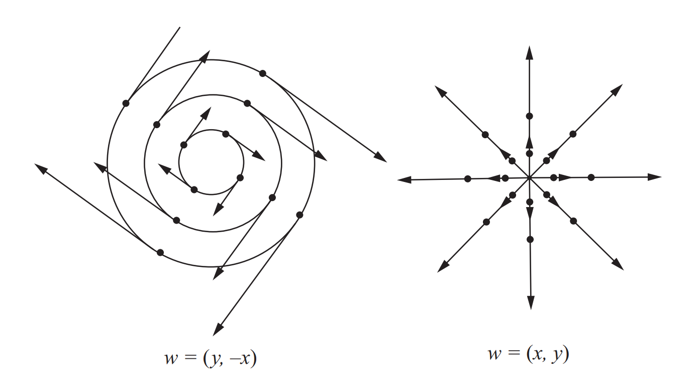
我们说向量场$w$决定了上面这样一个微分方程系统. 如对向量场$w(x,y)=(x,y),$
过$(x_0,y_0)$点的轨迹为$\alpha(t)=(x_0e^t,y_0 e^t);$
对向量场$w(x,y)=(y,-x),$
过$(x_0,y_0)$点轨迹为$\beta(t)=(r\sin t,r\cos t),$ $r^2=x_0^2+y_0^2.$
由常微分方程基本理论(存在性, 唯一性), 我们有如下定理:
定理 1.1. 对任意开集$U\subset \mathbb{R}^2$上给定向量场$w,$ 以及定点$p\in U,$ 存在场的轨迹$\alpha:I\rightarrow U,$ 其中$I$为原点处小邻域, $\alpha(0)=p.$ 这样的轨迹是唯一的, 即若有另一条轨迹$\beta:J\rightarrow U,$ $J$为原点小邻域, $\beta(0)=p,$ 则限制在$I\cap J$上$\alpha=\beta.$
又由解对初值的依赖性, 我们进一步有:
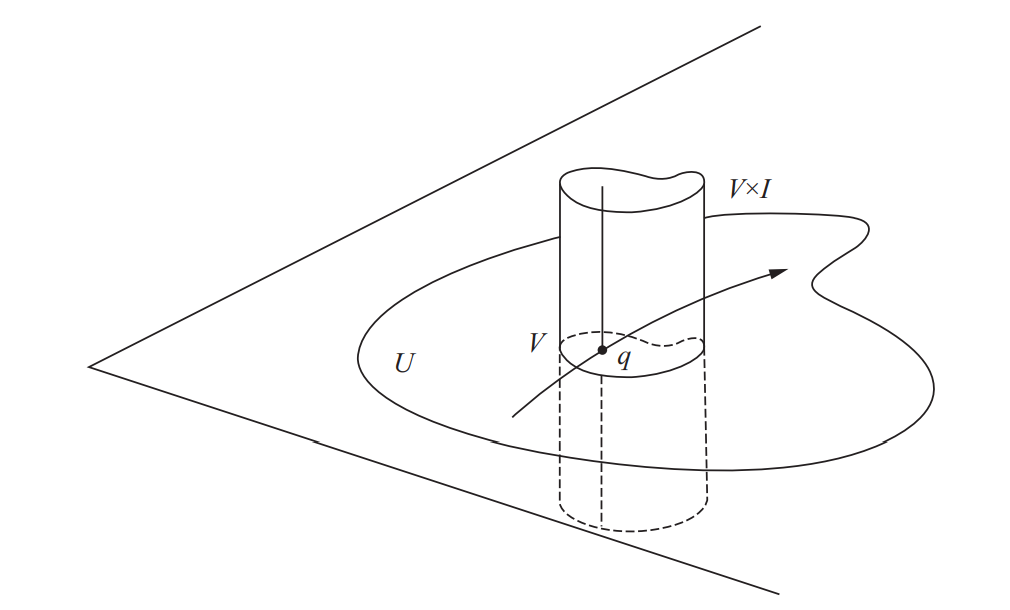
定理 1.2. 字母含义同上, 存在$p$点邻域$V\subset U\subset \mathbb{R}^2,$ 有可微映射$\alpha:V\times I\rightarrow U,$ 使得$\,\forall\,q\in V,$ $\alpha(q,\cdot)$为场$w$过$q$点的轨迹.
这样的映射$\alpha$称为$w$在$p$点的(局部)流(local flow). 从图示来看,
它将柱体\”拍\”到平面$(U)$上, 将每一根竖线映为轨迹.
由上述定理, 有结论如下:
引理 1.3. 令$w$为开集$U\subset \mathbb{R}^2$上向量场, $p\in U$有$w(p)\neq 0.$ 那么存在$p$点邻域$W\subset U$与可微函数$f:W\rightarrow \mathbb{R},$ 使得$f$沿轨迹为常数, 且$df_q\neq 0,$ $\,\forall\,q\in W.$
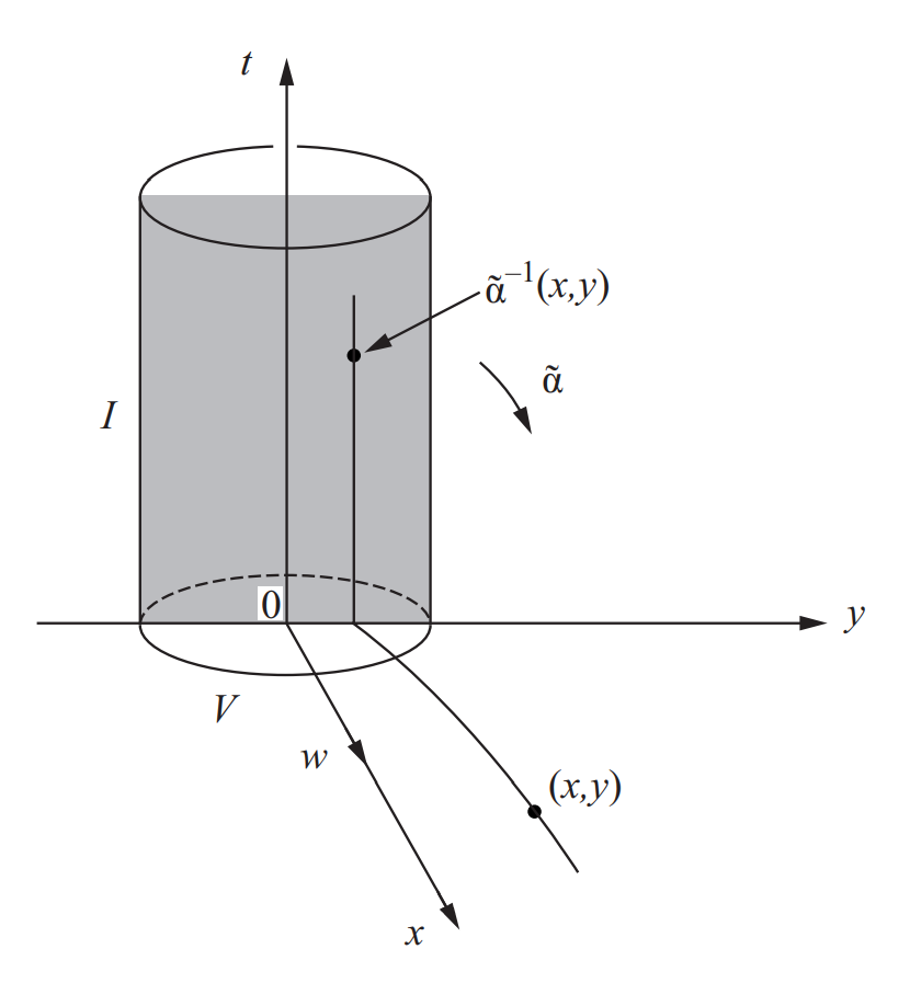
证: 不妨设$p$为原点, $w(p)$沿$x$轴方向.
由上述定理我们有局部流$\alpha:V\times I\rightarrow U.$
取$\tilde\alpha$为$\alpha$限制在矩形$(V\times I)\cap \{(0,y,t)\in \mathbb{R}^3\}$上.
由定义, $d\tilde \alpha_p$将$t$轴切方向映到$w(p),$
将$y$轴切方向映到自身, 因此$d\tilde \alpha_p$不退化. 由反函数定理,
在充分小的邻域$W\subset U$上, 存在可微函数$\tilde \alpha^{-1}.$
那么取$f$为$\tilde \alpha^{-1}$在$y$轴上的分量即可. 易见$f$满足要求.
这样的沿轨迹(解)为常数的函数$f$称为场$w$在$p$点邻域的(局部)首次积分.
如对场$w(x,y)=(y,-x),$
在$\mathbb{R}^2-O$上的一个首次积分是$f(x,y)=x^2+y^2.$
容易看出这样定义的首次积分并不唯一. 由隐函数定理, 在$f$微分不消失的地方,
$f=C$就给出了$x,y$的关系, 从而消去一个未知量, 使求解变得容易.
开集$U\subset \mathbb{R}^2$上的方向场$r,$ 指对每个点$p\in U,$
在$\mathbb{R}^2$上指定一条过$p$点的直线$r(p).$ 称$r$是在$p$点可微的,
若$p$点邻域$V\subset U$上存在一个非零可微向量场$w,$
满足$\,\forall\,q\in V$, 非零的$w(q)$为$r(q)$的基.
$r$在$U$上可微自然指在$U$上点点可微.
每个非零可微向量场$w$自然可以生成一个可微方向场$r.$
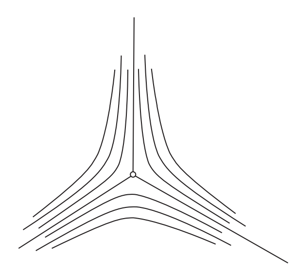
需要注意的是, 根据定义, 每个可微方向场点点局部对应一个非零可微向量场$w,$
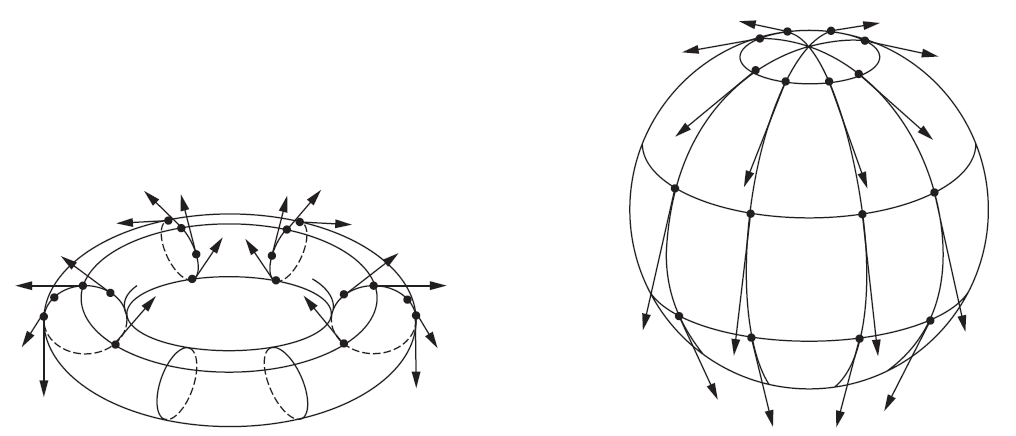
但不见得整体对应一个非零可微向量场, 如下图所示.
可以说方向场对应的向量场局部给出了方向场的一个定向,
那么无法整体定向的方向场也就不能对应一个整体非零的向量场了.
一个正则曲线$C\subset U$称为$U$上方向场$r$的积分曲线,
若$\,\forall\,q\in C,$ $r(q)$为$C$在$q$点切线.
易见积分曲线局部上就是可微方向场所对应的向量场的轨迹,
由此每个可微方向场总能找到过任意定点的积分曲线,
即类似于常微分方程中解的拼接, 积分曲线就是将向量场的轨迹拼接起来.
既然轨迹与积分曲线看似对应的是同一个东西, 为何要引入新的定义呢?
因为整体的方向场不见得对应整体的向量场, 因此没有所谓整体的轨迹这一概念,
但整体的积分曲线是确实存在的. 可见可微性之于方向场也很重要,
我们默认总是考虑可微的方向场.
方向场也可由微分方程给出. 对任意向量场$w,$
易见$\,\forall\,\lambda\neq 0,$ $\lambda w$与$w$生成的方向场是一致的,
$\lambda$可以是一个处处非零的可微函数. 对常微分方程组$\begin{cases}
\frac{dx}{dt}=\lambda(x,y)a(x,y)\\ \frac{dy}{dt}=\lambda(x,y)b(x,y)
\end{cases},$ 为了消去$\lambda,$
可以由微分方程$b(x,y)\frac{dx}{dt}-a(x,y)\frac{dy}{dt}=0$表示该方向场,
方程的解就对应着积分曲线.
对方向场我们不在乎曲线的参数化(对向量场的轨迹需要注意参数选取),
因此我们常用形如$adx+bdy=0$的微分方程来表示方向场.
曲面上的向量场
前面的所有内容仅用到了$\mathbb{R}^2$上的局部性质, 主要依赖于其可微结构.
因此我们自然可以把上述讨论迁移到曲面上.
定义 1.4. 曲面$S$中开集$U$上的向量场$w,$ 为对每个点$p\in U,$ 指定一个$w(p)\in T_p(S)$的对应. 称其在$p$点可微, 若对$p$点某邻域上的参数化$x(u,v),$ 存在可微的$a(u,v), b(u,v),$ 使得$w(x(u,v))=a(u,v)x_u+b(u,v)x_v.$ 它与参数化选取无关.
类似的, 可定义向量场的轨迹, 方向场, 积分曲线等.
只需将$\mathbb{R}^2$换为$S$即可, 定理与引理也自然是成立的.
接下来介绍本节的主定理.
定理 1.5. 在开集$U\subset S$上有两向量场$w_1,w_2,$ 在某点$p\in U$处线性无关. 那么存在某$p$点邻域$V\subset U,$ 其上有参数化使得$\,\forall\,q\in V,$ 过该点的两条坐标曲线分别与$w_1(q),w_2(q)$相切.
证: 取$p$点邻域$W\subset U,$ 使其上有首次积分$f_1,f_2.$
定义$\varphi:W\rightarrow \mathbb{R}^2,$ $\varphi(q)=(f_1(q),f_2(q)),$
则$d\varphi_p(w_1)=(0,(df_2)_p(w_1))\neq 0,$
$d\varphi_p(w_2)=((df_1)_p(w_2),0)\neq 0,$ 且线性无关,
$d\varphi_p$不退化. 因此$\varphi$为局部同胚,
从而取$\varphi$为更小的邻域$V\subset W$上的坐标函数即可.
坐标曲线$f_1(q)=const, f_2(q)=const$分别与$w_1(q),w_2(q)$相切.
需要注意的是, 定理并不表示坐标曲线的速度向量就是$w_1(q),w_2(q).$
事实上可以将上述定理表示为下面的形式.
推论 1.6. 在开集$U\subset S$上有两方向场$r_1,r_2,$ 在某点$p\in U$处, $r_1(p)\neq r_2(p).$ 那么存在某$p$点邻域$V\subset U,$ 其上有参数化使得$\,\forall\,q\in V,$ 过该点的两条坐标曲线分别为$r_1,r_2$的积分曲线.
定理可以说明正交参数化的存在性:
推论 1.7. $\,\forall\,p\in S,$ $p$点某邻域$V$上存在参数化$x(u,v),$ 使得坐标曲线$u=const,v=const$在任意点$q\in V$上彼此正交. 称这样的$x$为正交参数化.
证: 在点$p$处任取参数化$\bar x:\bar U\rightarrow S,$
取向量场$w_1=\bar x_{\bar u},$
$w_2=-(\bar F/\bar E)\bar x_{\bar u}+\bar x_{\bar v}.$
那么$w_1\cdot w_2=-\bar F +\bar F=0,$ 在任意点$q$处.
应用定理即得所需的参数化.
不仅如此, 还可在$p$点任意指定两个正交方向, 生成需要的正交参数化. 特别地,
对特殊的参数化, 有如下推论:
推论 1.8. 在双曲点附近存在参数化, 使得坐标曲线构成渐近线网; 在非脐点附近存在(正交)参数化, 使得坐标曲线构成曲率线网.
证: 在双曲点附近, 满足$eg-f^2<0,$
由此可线性分解渐近线微分方程$e{u'}^2+2fu'v'+g{v'}^2=0$为$(Au'+Bv')(Au'+Dv')=0$的形式,
从而确定两个方向场, 其积分曲线即为渐近线. 从而由前面的推论即得结论.
在非脐点附近, 由于曲率线微分方程较为复杂, 由前面的推论,
不妨先取正交参数化使$F=0.$ 由于是非脐点, 可取到正交参数化使$f\neq 0,$
进而由$EGf^2>0,$ 同上面的方法可线性分解微分方程, 得到方向场,
积分曲线即为曲率线. 由前面的推论即得结论.
直纹面与极小曲面
直纹面
一个可微的单参数直线族$\{L_t\}$, 指有可微的$\{\alpha(t),w(t)\},$
对每个$t\in I,$ 指定一点$\alpha(t)\in \mathbb{R}^2$与向量$w(t).$
直线$L_t$过$\alpha(t),$ 以$w(t)$为方向.
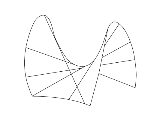
直纹面即为由单参数直线族生成的曲面, 即有$x(t,v)=\alpha(t)+vw(t),$
$(t,v)\in I\times \mathbb{R}.$ 直线$L_t$称为直母线(rulings),
曲线$\alpha(t)$称为曲面的准线(directrix). 一般来说, 允许$x$出现奇点.
接下来总是假设$|w(t)|=1,$ $w'(t)\neq 0.$ 后一假设即曲面是非柱状的.
由前一假设有$\left<{}w(t),w'(t)\right>=0.$
我们希望找到一条曲线$\beta(t)$使得$\left<{}\beta'(t),w'(t)\right>=0,$
且$\beta$落在$x$上. 设$\beta(t)=\alpha(t)+u(t)w(t),$
则$\beta'=\alpha'+u'w+uw'.$ 若满足要求,
则$0=\left<{}\beta',w'\right>=\left<{}\alpha',w'\right>+u\left<{}w',w'\right>,$
$u=-\frac{\left<{}\alpha',w'\right>}{\left<{}w',w'\right>}.$
从而取这样的$u$, 对应的$\beta$即满足要求.
接下来说明$\beta$与准线的选取无关.
若$x(t,u)=\alpha(t)+uw(t)=\bar\alpha(t)+v(u)w(t).$
那么$\beta-\bar \beta=(\alpha-\bar\alpha)+\frac{\left<{}\bar\alpha'-\alpha',w'\right>}{\left<{}w',w'\right>}w.$
由于$\alpha-\bar\alpha=(u-v)w,$ 且$\left<{}w,w'\right>=0,$
便有$\beta=\bar\beta.$ 从而这样的曲线$\beta$只与直纹面本身有关,
称其为腰线, 其上的点称为直纹面的中心点. 如螺旋面的腰线是中心轴,
而单叶双曲面的腰线是半径最小的纬线.\
选取$\beta$为直纹面的准线, $x(t,u)=\beta(t)+uw(t),$
那么$x_t=\beta'+uw',$ $x_u=w,$
$x_t\wedge x_u=\beta'\wedge w+uw'\wedge w.$ $w'$垂直于$\beta',w,$
从而可记$\beta'\wedge w=\lambda w',$ $\lambda=\lambda(t).$
那么$|x_t\wedge x_u|^2=(\lambda^2+u^2)|w'|^2,$
从而奇点只可能在$u=0$即准线$\beta$上出现. 且出现奇点当且仅当$\lambda=0,$
即$w(t)$在准线切线上.
可具体表示出$\lambda=\frac{(\beta',w,w')}{|w'|^2}.$
我们来计算直纹面在正则点处的Gauss曲率. $x_{tt}=\beta''+uw'',$
$x_{tu}=w',$ $x_{uu}=0,$ 从而$g=0,$
$f=\frac{(x_t,x_u,x_{tu})}{|x_t\wedge x_u|}=\frac{(\beta',w,w')}{|x_t\wedge x_u|}.$
故$K=\frac{eg-f^2}{EG-F^2}=-\frac{\lambda^2 |w'|^4}{(\lambda^2+u^2)^2|w'|^4}=-\frac{\lambda^2}{(\lambda^2+u^2)^2}.$
从而在正则点, 直纹面的Gauss曲率$K\le 0,$
且等于零仅当$w(t)$落在$\beta(t)$切线上, 沿该直母线发生. 可以看出,
若$\lambda\neq 0,$ 则$|K(u)|$是直母线上的连续函数, 取值关于中心点对称,
在中心点处$|K(u)|$达到极大值.
函数$\lambda(t)$称为$x$的分布参数. 由于腰线与准线选取无关,
$\lambda$也是. 若$x$是正则的,
有$N(t,u)=\frac{x_t\wedge x_u}{|x_t\wedge x_u|}=\frac{\lambda w'+uw'\wedge w}{\sqrt{\lambda^2+u^2}|w'|}.$
若$\lambda\neq 0,$ $N(t,0)=\frac{w'}{|w'|}\frac{\lambda}{|\lambda|}.$
考虑$N(t,u)$与$N(t,0)$夹角, $\tan\theta=\frac{u}{|\lambda|},$
与$u$成正比, 比例系数为分布参数的倒数.
利用这一性质, 可以推出一个有趣的结论是,
由直母线上法向量对应的单参数直线族, 生成的直纹面恰为双曲抛物面$z=kxy,$
$k=\frac{1}{\lambda}.$
对直纹面$x(t,v)=\alpha(t)+vw(t),$ 称它是可展的,
若$(\alpha',w,w')=0.$ 计算得到$g=0,$
$f=\frac{(\alpha',w,w')}{|x_t\wedge x_u|}=0,$
从而$K=\frac{eg-f^2}{EG-F^2}=0,$ 即可展曲面Gauss曲率恒为零.
事实上反过来也是对的, 即Gauss曲率为零的曲面也一定是可展的.
它与平面局部等距, 因此可以剪下曲面上的一块展开为平面,
这也是可展曲面得名的原因.
一个基本的事实是可展曲线的切平面沿直母线不变.
只需说明$\left<{}N_v,x_v\right>=\left<{}N_v,x_t\right>=0,$ 即$f=g=0.$
这是已经得到过的.\
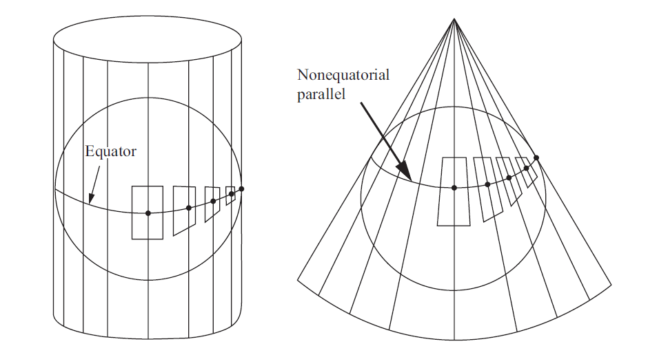
接下来我们说明可展曲面只有柱面, 锥面, 切线面这三类.
$w'=0$的部分为柱状区域, 去掉$w'=0$的部分后, 曲面是非柱状的.
由前面的讨论, 可取到腰线$\beta(t),$ 且分布参数$\lambda=0,$
从而腰线上都是奇点. 在$\beta'=0$的地方, 该点处的曲面为锥面;
去掉$\beta'=0$的地方后, 由$\lambda=0$得到$\beta'$与$w$同向,
即曲面为切线面.
可展曲面的一个重要性质, 或者说等价的定义方式是,
它是单参数平面族的包络面. 取正则曲面$S$与其上的弧长参数化曲线$\alpha,$
假设它无处切方向是渐进的. 记$N(s)=N\circ\alpha(s),$
那么$\left<{}dN(\alpha'),\alpha'\right>=\left<{}N',\alpha'\right>\neq 0,$
从而$N'\neq 0.$
取直纹面$x(s,v)=\alpha(s)+v\frac{N(s)\wedge N'(s)}{|N'(s)|}.$
考虑沿$\alpha(s)$的$S$的切平面族$\{T_{\alpha(s)}(S)\},$
很近的两平面交于某直线,
以$\frac{N(s)\wedge N(s+\Delta s)}{\Delta s}$为方向.
令$\Delta s\rightarrow 0$即有该方向为$N\wedge N'.$
从而$x$的直母线为平面族邻近平面交线的极限.
这样的$x$即称为单参数平面族$\{T_{\alpha(s)}(S)\}$的包络面.
柱面和锥面很显然可由该种方法生成.
可以很直接的计算出,
$(\alpha',w,w')=\frac{1}{|N'|^2}\left<{}(N\wedge N')\wedge (N\wedge N')',\alpha'\right>=\frac{1}{|N'|^2}\left<{}\left<{}N\wedge N',N''\right>N,\alpha'\right>=0,$
从而单参数平面族包络面可展. 对可展曲面,
也能够找到对应的单参数平面族以其为包络面.
接下来我们说明$x$在$\alpha$附近正则, 且沿$\alpha$与$S$相切.在$\alpha$上,
$x_s\wedge x_v=\alpha'\wedge\frac{N\wedge N'}{|N'|}=\left<{}N',\alpha'\right>\frac{N}{|N'|}=-\frac{k_nN}{|N'|}.$
由于$\alpha'$非渐进方向, $k_n$无处为零, 从而$x$在$\alpha$附近正则,
且在$\alpha$处法向量与$S$一致, 即与$S$相切.
极小曲面
一个正则参数化曲面是极小的, 若其平均曲率处处消失.
令$x:U\subset \mathbb{R}^2\rightarrow \mathbb{R}^3$为正则参数化曲面.
取有界区域$D\subset U,$ 以及可微函数$h:\bar D\rightarrow \mathbb{R}.$
$x(\bar D)$由$h$决定的法向变分,
指映射$\varphi:\bar D\times (-\varepsilon,\varepsilon)\rightarrow \mathbb{R}^3,$
$\varphi(u,v,t)=x(u,v)+th(u,v)N(u,v).$
对每个固定的$t\in (-\varepsilon,\varepsilon),$
$x^t:D\rightarrow \mathbb{R}^3,$
$x^t(u,v)=\varphi(u,v,t)$为一个参数化曲面. 计算得到$I^t=I-2thII+o(t).$
由平均曲率$H=\frac{1}{2}\frac{Eg-2fF+Ge}{EG-F^2},$
可以得到$E^tG^t-(F^t)^2=(EG-F^2)(1-4thH)+o(t).$
从而$x^t(\bar D)$曲面面积$A(t)=\int_{\bar D}\sqrt{1-4thH+o(t)}\sqrt{EG-F^2}dudv,$
对充分小的$\varepsilon$为可微函数,
且在零点导数$A'(0)=\int_{\bar D}-2hH \sqrt{EG-F^2}dudv.$
命题 1.9. 条件同上, $x$为极小曲面当且仅当$A'(0)=0$对任意法向变分成立.
证: 必要性易见. 假设$H(q)\neq 0,$
取支撑在点$q$充分小邻域上的$h:\bar D\rightarrow \mathbb{R}$使得$h(q)=H(q),$
$hH>0.$ 那么对于该$h$决定的法向变分, $A'(0)<0,$ 矛盾.
需要注意的是, 其实我们只说明了极小曲面面积达到临界值, 未必真的是极小值.
但极小曲面这一定义由Lagrange早在1760年便提出, 因此一直沿用至今.
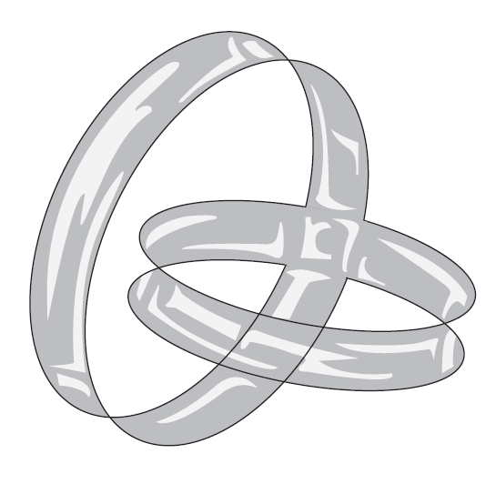
提到极小曲面往往会提到皂膜. 给定一个框架, 将其放入肥皂水中,
小心翼翼的拿出来, 框架上便会架起皂膜. 这些皂膜便是面积达到极小的曲面,
这样我们就制造出了极小曲面.
一般的, 定义平均曲率向量为$H=HN,$ 令$h=H$,
那么$A'(0)=\int_{\bar D}-2\left<{}H,H\right>\sqrt{EG-F^2}dudv<0,$
也就是沿着平均曲率向量, 面积在零点附近是递减的.
对等温曲面, 即$E=G=\lambda^2,$ $F=0,$ 有如下命题:
命题 1.10. 设$x(u,v)$为正则参数化等温曲面, 那么$x_{uu}+x_{vv}=2\lambda^2 H.$
证: 首先由微分, 有:
$\left<{}x_{uu},x_u\right>=\left<{}x_{vu},x_v\right>=-\left<{}x_u,x_{vv}\right>,$
从而$\left<{}x_{uu}+x_{vv},x_u\right>=0.$
类似的$\left<{}x_{uu}+x_{vv},x_v\right>=0.$
从而$x_{uu}+x_{vv}$沿$N$方向.
计算得到平均曲率$H=\frac{1}{2}\frac{g+e}{\lambda^2}.$ 因此,
$2\lambda^2 H=g+e=\left<{}N,x_{uu}+x_{vv}\right>,$
从而$x_{uu}+x_{vv}=2\lambda^2 H.$
推论 1.11. 对正则参数化等温曲面$x(u,v)=(x(u,v),y(u,v),z(u,v)),$ $x$极小当且仅当坐标分量都是调和的.
关于极小曲面有若干经典的例子. 如悬链面是旋转面中唯一的极小曲面,
通过取旋转面的参数化计算即可. 这一点并不难以理解,
极小曲面和悬链线都是自然形成的,
因此有理由相信悬链线形成的悬链面是极小曲面.
另一个例子是螺旋面是直纹面中唯一的极小曲面, 除了平面.
教材中引用了Osserman的survey中,
极小曲面Gauss曲率零点孤立这一性质(平面除外).
除去Gauss曲率取零点的地方, 由于平均曲率为零, Gauss曲率必然取负.
由于$k_1=-k_2,$ 由Euler公式, 曲面有正交的渐进曲线. 显然直母线是渐进曲线,
由于曲面非平面, 可取到点$q\in W,$
过该点的另一条渐进曲线以$\tau=\sqrt{-K}$为挠率.
由于渐进曲线密切平面为曲面切平面,
在$q$点邻域$V\subset W$上直母线恰为另一渐进曲线族的法线.
这当且仅当该曲线族为螺线族时发生(Bertrand曲线), 因此$V$是螺面的一部分.
由于螺线挠率恒定, 可见整个曲面都是螺旋面.
极小曲面是微分几何中重要的研究课题, 许多有关它的结论都很形象,
但又相当难以证明. 书中提到如下的定理:
定理 1.12. 令$S$为非平面的正则极小闭曲面, 那么Gauss映射像在球面上是稠密的.
文章最后更新于 2021-08-25 10:50:16
vector field
Vector field on the plane
On the open set $U\subset \mathbb{R}^2$ vector field is a mapping,
For each $q=(x,y)\in U$, specify an $w(q)=(a(x,y),b(x,y))\in \mathbb{R}^2.$
The vector field is said to be Differentiable, if $w$ is differentiable, that is, $a,b$ is all differentiable.
By default we always consider differentiable vector fields.
Given a vector field, we consider whether there is a trajectory,
That is, whether there is a differentiable curve $\alpha(t)=(x(t),y(t)),$
so that $\alpha'(t)=w(\alpha(t)).$ In fact, this is the solution of the system of ordinary differential equations: $$\left\{
\begin{aligned}
\frac{dx}{dt}=a(x,y)\\
\frac{dy}{dt}=b(x,y)
\end{aligned}
\right.$$
We say that the vector field $w$ determines the above system of differential equations. For example, the vector field $w(x,y)=(x,y),$
The trajectory passing through point $(x_0,y_0)$ is $\alpha(t)=(x_0e^t,y_0 e^t);$
Pair vector field$w(x,y)=(y,-x),$
The trajectory passing $(x_0,y_0)$ point is $\beta(t)=(r\sin t,r\cos t),$ $r^2=x_0^2+y_0^2.$
From the basic theory of ordinary differential equations (existence, uniqueness), we have the following theorem:
Theorem 1.1. For a given vector field $w,$ and a fixed point $p\in U,$ on any open set $U\subset \mathbb{R}^2$, there is a field trajectory $\alpha:I\rightarrow U,$ where $I$ is a small neighborhood at the origin, $\alpha(0)=p.$ such a trajectory is unique, that is, if there is another trajectory $\beta:J\rightarrow U,$ $J$ is a small neighborhood at the origin, $\beta(0)=p,$ is limited to $I\cap J$ $\alpha=\beta.$
Based on the dependence of the solution on the initial value, we further have:
Theorem 1.2. The meaning of the letters is the same as above. There is a $p$ point neighborhood $V\subset U\subset \mathbb{R}^2,$ and a differentiable mapping $\alpha:V\times I\rightarrow U,$ such that $\,\forall\,q\in V,$ $\alpha(q,\cdot)$ is the trajectory of the field $w$ passing through the $q$ point.
Such a mapping $\alpha$ is called (local) of $w$ at point $p$ flow (local flow). From the diagram,
It "shoots" the cylinder onto the plane $(U)$, mapping each vertical line as a trajectory.
From the above theorem, the conclusion is as follows:
Lemma 1.3. Let $w$ be the vector field on the open set $U\subset \mathbb{R}^2$, $p\in U$ has $w(p)\neq 0.$, then there exists $p$ point neighborhood $W\subset U$ and differentiable function $f:W\rightarrow \mathbb{R},$ such that $f$ is constant along the trajectory, and $df_q\neq 0,$ $\,\forall\,q\in W.$
Certificate: Let’s set $p$ as the origin and $w(p)$ along the $x$ axis.
From the above theorem we have local flow $\alpha:V\times I\rightarrow U.$
Take $\tilde\alpha$ as $\alpha$ and limit it to the rectangle $(V\times I)\cap \{(0,y,t)\in \mathbb{R}^3\}$.
By definition, $d\tilde \alpha_p$ maps the axis tangent direction of $t$ to $w(p),$
Reflect the tangent direction of the $y$ axis to itself, so $d\tilde \alpha_p$ does not degenerate. According to the inverse function theorem,
On a sufficiently small neighborhood $W\subset U$, there is a differentiable function $\tilde \alpha^{-1}.$
Then take $f$ as the component of $\tilde \alpha^{-1}$ on the $y$ axis. It is easy to see that $f$ meets the requirements.
Such a function $f$ that is constant along the trajectory (solution) is called the (local) first integral of the field $w$ in the neighborhood of the point $p$.
Such as on the field $w(x,y)=(y,-x),$
A first point on $\mathbb{R}^2-O$ is $f(x,y)=x^2+y^2.$
It is easy to see that the first integral defined in this way is not unique. According to the implicit function theorem, where $f$ the differential does not disappear,
$f=C$ gives the relationship of $x,y$, thus eliminating an unknown quantity and making the solution easier.
On the open set $U\subset \mathbb{R}^2$ direction field $r,$ refers to each point $p\in U,$
Specify a straight line $r(p).$ passing $p$ point on $\mathbb{R}^2$. It is said that $r$ is at the $p$ point. Differentiable,
If there is a non-zero differentiable vector field $w,$ in the neighborhood $V\subset U$ of the point $p$
Satisfying $\,\forall\,q\in V$, non-zero $w(q)$ is the basis of $r(q)$.
$r$ being differentiable on $U$ naturally means that it is slightly differentiable on $U$.
Each non-zero differentiable vector field $w$ naturally generates a differentiable direction field $r.$
It should be noted that, according to the definition, each differentiable direction field point locally corresponds to a non-zero differentiable vector field $w,$
But it does not necessarily correspond to a non-zero differentiable vector field as a whole, as shown in the figure below.
It can be said that the vector field corresponding to the direction field locally gives an orientation of the direction field,
Then a direction field that cannot be oriented as a whole cannot correspond to an overall non-zero vector field.
A regular curve $C\subset U$ is called the direction field $r$ above $U$. integral curve,
If $\,\forall\,q\in C,$ $r(q)$ is tangent to $C$ at point $q$.
It is easy to see that the integral curve is locally the trajectory of the vector field corresponding to the differentiable direction field,
Therefore, each differentiable direction field can always find the integral curve passing through any fixed point,
That is, similar to the splicing of solutions in ordinary differential equations, the integral curve is to splice the trajectories of the vector fields together.
Since the trajectory and the integral curve seem to correspond to the same thing, why introduce a new definition?
Because the overall direction field does not necessarily correspond to the overall vector field, there is no concept of the so-called overall trajectory.
But the overall integral curve does exist. It can be seen that differentiability is also very important for the direction field.
By default we always consider differentiable direction fields.
The direction field can also be given by a differential equation. For any vector field $w,$
It is easy to see that the direction fields generated by $\,\forall\,\lambda\neq 0,$ $\lambda w$ and $w$ are consistent.
$\lambda$ can be a differentiable function that is non-zero everywhere. For a system of ordinary differential equations $\begin{cases}
\frac{dx}{dt}=\lambda(x,y)a(x,y)\\ \frac{dy}{dt}=\lambda(x,y)b(x,y)
\end{cases},$, in order to eliminate $\lambda,$
This direction field can be expressed by the differential equation $b(x,y)\frac{dx}{dt}-a(x,y)\frac{dy}{dt}=0$,
The solution to the equation corresponds to the integral curve.
For the direction field, we don’t care about the parameterization of the curve (for the trajectory of the vector field, we need to pay attention to parameter selection),
Therefore, we often use differential equations of the form $adx+bdy=0$ to express the direction field.
vector field on a surface
All the previous content only uses the local properties on $\mathbb{R}^2$, mainly relying on its differentiable structure.
Therefore, we can naturally transfer the above discussion to the surface.
Definition 1.4. The vector field $w,$ on the open set $U$ in the surface $S$ specifies a correspondence to $w(p)\in T_p(S)$ for each point $p\in U,$. It is said to be differentiable at the $p$ point. If there is a differentiable $a(u,v), b(u,v),$ for the parameterization $x(u,v),$ on a certain neighborhood of the $p$ point, making $w(x(u,v))=a(u,v)x_u+b(u,v)x_v.$ irrelevant to the parameterization selection.
Similarly, you can define the trajectory of the vector field, the direction field, the integral curve, etc.
Just replace $\mathbb{R}^2$ with $S$, and the theorem and lemma will naturally be established.
Next, we introduce the main theorem of this section.
Theorem 1.5. There are two vector fields $w_1,w_2,$ on the open set $U\subset S$ that are linearly independent at a certain point $p\in U$. Then there is a certain $p$ point neighborhood $V\subset U,$ on which there is parameterization such that the two coordinate curves $\,\forall\,q\in V,$ passing through the point are tangent to $w_1(q),w_2(q)$ respectively.
Certificate: Take $p$ point neighborhood $W\subset U,$ so that it has the first integral $f_1,f_2.$
Definition $\varphi:W\rightarrow \mathbb{R}^2,$ $\varphi(q)=(f_1(q),f_2(q)),$
Then $d\varphi_p(w_1)=(0,(df_2)_p(w_1))\neq 0,$
$d\varphi_p(w_2)=((df_1)_p(w_2),0)\neq 0,$ and linearly independent,
$d\varphi_p$ does not degenerate. Therefore $\varphi$ is a local homeomorphism,
Therefore, $\varphi$ can be taken as the coordinate function on the smaller neighborhood $V\subset W$.
The coordinate curves $f_1(q)=const, f_2(q)=const$ are tangent to $w_1(q),w_2(q)$ respectively.
It should be noted that the theorem does not mean that the velocity vector of the coordinate curve is $w_1(q),w_2(q).$
In fact, the above theorem can be expressed in the following form.
Corollary 1.6. On the open set $U\subset S$, there are two directional fields $r_1,r_2,$ at a certain point $p\in U$, $r_1(p)\neq r_2(p).$, then there is a certain $p$ point neighborhood $V\subset U,$ on which there is parameterization such that the two coordinate curves $\,\forall\,q\in V,$ passing through the point are integral curves of $r_1,r_2$ respectively.
The theorem can illustrate the existence of orthogonal parameterization:
Corollary 1.7. $\,\forall\,p\in S,$ $p$ There is a parameterization $x(u,v),$ on a certain neighborhood $V$ of the point such that the coordinate curves $u=const,v=const$ are orthogonal to each other at any point $q\in V$. Such a $x$ is called an orthogonal parameterization.
Certificate: Take any parameterization $\bar x:\bar U\rightarrow S,$ at point $p$
Orientation vector field $w_1=\bar x_{\bar u},$
$w_2=-(\bar F/\bar E)\bar x_{\bar u}+\bar x_{\bar v}.$
Then $w_1\cdot w_2=-\bar F +\bar F=0,$ is at any point $q$.
Applying the theorem yields the required parameterization.
Not only that, you can also arbitrarily specify two orthogonal directions at the $p$ point to generate the required orthogonal parameterization. In particular,
For special parameterizations, we have the following corollary:
Corollary 1.8. There is parameterization near the hyperbolic point, so that the coordinate curve forms an asymptote network; there is (orthogonal) parameterization near the non-umbilical point, so that the coordinate curve forms a curvature line network.
Certificate: Near the hyperbolic point, satisfies $eg-f^2<0,$
From this, the asymptote differential equation $e{u'}^2+2fu'v'+g{v'}^2=0$ can be linearly decomposed into the form $(Au'+Bv')(Au'+Dv')=0$,
Thus, the two direction fields are determined, and their integral curves are the asymptotes. The conclusion can be drawn from the previous inference.
Near the non-umbilical point, since the differential equation of the curvature line is more complicated, from the previous inference,
We might as well take the orthogonal parameterization $F=0.$ first. Since it is a non-umbilical point, we can take the orthogonal parameterization $f\neq 0,$
Then the differential equation can be linearly decomposed using the same method as above $EGf^2>0,$ to obtain the direction field,
The integral curve is the curvature line. The conclusion can be drawn from the previous inference.
Ruled surfaces and minimally curved surfaces
Ruled surface
A differentiable single-parameter straight line family $\{L_t\}$ refers to a differentiable $\{\alpha(t),w(t)\},$
For each $t\in I,$, specify a point $\alpha(t)\in \mathbb{R}^2$ and a vector $w(t).$
The straight line $L_t$ passes through $\alpha(t),$ with $w(t)$ as the direction.
A ruled surface is a surface generated by a single-parameter straight line family, that is, $x(t,v)=\alpha(t)+vw(t),$
$(t,v)\in I\times \mathbb{R}.$ Straight lines $L_t$ are called straight buses (rulings),
Curve $\alpha(t)$ is called the directrix of the surface. Generally speaking, singular points are allowed to occur in $x$.
Next always assume $|w(t)|=1,$ $w'(t)\neq 0.$ The latter assumption is that the surface is non-cylindrical.
From the previous assumption, we have $\left<{}w(t),w'(t)\right>=0.$
We hope to find a curve $\beta(t)$ such that $\left<{}\beta'(t),w'(t)\right>=0,$
And $\beta$ falls on $x$. Let $\beta(t)=\alpha(t)+u(t)w(t),$
Then $\beta'=\alpha'+u'w+uw'.$ if it meets the requirements,
Then $0=\left<{}\beta',w'\right>=\left<{}\alpha',w'\right>+u\left<{}w',w'\right>,$
$u=-\frac{\left<{}\alpha',w'\right>}{\left<{}w',w'\right>}.$
Therefore, taking $u$ like this, the corresponding $\beta$ meets the requirements.
Next, it will be explained that $\beta$ has nothing to do with the selection of the directrix.
If$x(t,u)=\alpha(t)+uw(t)=\bar\alpha(t)+v(u)w(t).$
Then $\beta-\bar \beta=(\alpha-\bar\alpha)+\frac{\left<{}\bar\alpha'-\alpha',w'\right>}{\left<{}w',w'\right>}w.$
Since $\alpha-\bar\alpha=(u-v)w,$ and $\left<{}w,w'\right>=0,$
There is $\beta=\bar\beta.$, so such a curve $\beta$ is only related to the ruled surface itself,
call it Waistline, the points on it are called ruled surfaces center point. For example, the waist line of the spiral surface is the central axis,
The waist line of a single-leaf hyperboloid is the latitude line with the smallest radius.\
Select $\beta$ as the directrix of the ruled surface, $x(t,u)=\beta(t)+uw(t),$
Then $x_t=\beta'+uw',$ $x_u=w,$
$x_t\wedge x_u=\beta'\wedge w+uw'\wedge w.$ $w'$ perpendicular to $\beta',w,$
So you can remember $\beta'\wedge w=\lambda w',$ $\lambda=\lambda(t).$
Then $|x_t\wedge x_u|^2=(\lambda^2+u^2)|w'|^2,$
Therefore, the singular point can only appear on $u=0$, that is, the directrix $\beta$. And the singular point appears if and only if $\lambda=0,$
That is, $w(t)$ is on the tangent to the directrix.
Can be expressed specifically $\lambda=\frac{(\beta',w,w')}{|w'|^2}.$
Let's calculate the Gauss curvature of the ruled surface at the regular point. $x_{tt}=\beta''+uw'',$
$x_{tu}=w',$ $x_{uu}=0,$ thus $g=0,$
$f=\frac{(x_t,x_u,x_{tu})}{|x_t\wedge x_u|}=\frac{(\beta',w,w')}{|x_t\wedge x_u|}.$
Therefore$K=\frac{eg-f^2}{EG-F^2}=-\frac{\lambda^2 |w'|^4}{(\lambda^2+u^2)^2|w'|^4}=-\frac{\lambda^2}{(\lambda^2+u^2)^2}.$
Therefore, at the regular point, the Gauss curvature of the ruled surface $K\le 0,$
And equal to zero only when $w(t)$ falls on the tangent line $\beta(t)$, occurs along the straight bus. It can be seen that,
If $\lambda\neq 0,$ then $|K(u)|$ is a continuous function on the straight bus, and its value is symmetrical about the center point,
At the center point $|K(u)|$ reaches the maximum value.
The function $\lambda(t)$ is called the distribution parameter of $x$. Since the waistline has nothing to do with the selection of the directrix,
The same goes for $\lambda$. If $x$ is regular,
Yes $N(t,u)=\frac{x_t\wedge x_u}{|x_t\wedge x_u|}=\frac{\lambda w'+uw'\wedge w}{\sqrt{\lambda^2+u^2}|w'|}.$
If $\lambda\neq 0,$ $N(t,0)=\frac{w'}{|w'|}\frac{\lambda}{|\lambda|}.$
Consider the angle between $N(t,u)$ and $N(t,0)$, $\tan\theta=\frac{u}{|\lambda|},$
Proportional to $u$, the proportional coefficient is the reciprocal of the distribution parameter.
Using this property, an interesting conclusion can be drawn:
The ruled surface generated by the single-parameter straight line family corresponding to the normal vector on the straight bus is exactly a hyperbolic parabola $z=kxy,$
$k=\frac{1}{\lambda}.$
For the ruled surface $x(t,v)=\alpha(t)+vw(t),$, call it Expandable,
If $(\alpha',w,w')=0.$ is calculated, $g=0,$
$f=\frac{(\alpha',w,w')}{|x_t\wedge x_u|}=0,$
Therefore $K=\frac{eg-f^2}{EG-F^2}=0,$ means that the Gauss curvature of the developable surface is always zero.
In fact, the reverse is also true, that is, a surface with zero Gauss curvature must also be developable.
It is locally equidistant from the plane, so you can cut a piece of the surface and expand it into a plane,
This is also the reason why developable surfaces are named.
A basic fact is that the tangent plane of a developable curve remains unchanged along the straight generator.
Just state that $\left<{}N_v,x_v\right>=\left<{}N_v,x_t\right>=0,$ is $f=g=0.$
This has been obtained.\
Next, we explain that there are only three types of developable surfaces: cylinder, cone, and tangent surface.
The $w'=0$ part is a columnar area. After removing the $w'=0$ part, the surface is non-columnar.
From the previous discussion, it can be obtained that the waistline $\beta(t),$ and the distribution parameter $\lambda=0,$
Therefore, all the waistlines are singular points. At $\beta'=0$, the surface at this point is a cone;
After removing $\beta'=0$, we can get $\beta'$ and $w$ in the same direction from $\lambda=0$.
That is, the surface is a tangent surface.
An important property of a developable surface, or the equivalent definition is,
It is the envelope surface of the single-parameter plane family. Take the regular surface $S$ and the arc length parameterized curve $\alpha,$ on it
Assume that its direction is asymptotic. Note $N(s)=N\circ\alpha(s),$
Then $\left<{}dN(\alpha'),\alpha'\right>=\left<{}N',\alpha'\right>\neq 0,$
Thus $N'\neq 0.$
Take the ruled surface $x(s,v)=\alpha(s)+v\frac{N(s)\wedge N'(s)}{|N'(s)|}.$
Consider the tangent plane family $\{T_{\alpha(s)}(S)\},$ of $S$ along $\alpha(s)$
Two very close planes intersect at a straight line,
Take $\frac{N(s)\wedge N(s+\Delta s)}{\Delta s}$ as the direction.
Let $\Delta s\rightarrow 0$ mean that the direction is $N\wedge N'.$
Therefore, the straight busbar of $x$ is the limit of the intersection of adjacent planes of the plane family.
Such $x$ is called the envelope surface of the single-parameter plane family $\{T_{\alpha(s)}(S)\}$.
Cylindrical and conical surfaces can obviously be generated by this method.
It can be calculated very directly,
$(\alpha',w,w')=\frac{1}{|N'|^2}\left<{}(N\wedge N')\wedge (N\wedge N')',\alpha'\right>=\frac{1}{|N'|^2}\left<{}\left<{}N\wedge N',N''\right>N,\alpha'\right>=0,$
Therefore, the envelope surface of the single-parameter plane family is developable. For a developable surface,
It is also possible to find the corresponding single-parameter plane family and use it as the envelope surface.
Next, we explain that $x$ is regular near $\alpha$ and is tangent to $S$ along $\alpha$. On $\alpha$,
$x_s\wedge x_v=\alpha'\wedge\frac{N\wedge N'}{|N'|}=\left<{}N',\alpha'\right>\frac{N}{|N'|}=-\frac{k_nN}{|N'|}.$
Since $\alpha'$ is a non-asymptotic direction, $k_n$ is zero everywhere, so $x$ is regular near $\alpha$,
And the normal vector at $\alpha$ is consistent with $S$, that is, tangent to $S$.
minimal surface
A regular parametric surface is extremely small, if its mean curvature disappears everywhere.
Let $x:U\subset \mathbb{R}^2\rightarrow \mathbb{R}^3$ be a regular parameterized surface.
Take the bounded area $D\subset U,$ and the differentiable function $h:\bar D\rightarrow \mathbb{R}.$
$x(\bar D)$ determined by $h$ normal variation,
Refers to mapping $\varphi:\bar D\times (-\varepsilon,\varepsilon)\rightarrow \mathbb{R}^3,$
$\varphi(u,v,t)=x(u,v)+th(u,v)N(u,v).$
For each fixed $t\in (-\varepsilon,\varepsilon),$
$x^t:D\rightarrow \mathbb{R}^3,$
$x^t(u,v)=\varphi(u,v,t)$ is a parametric surface. Calculate $I^t=I-2thII+o(t).$
From the mean curvature $H=\frac{1}{2}\frac{Eg-2fF+Ge}{EG-F^2},$
Can get $E^tG^t-(F^t)^2=(EG-F^2)(1-4thH)+o(t).$
Thus $x^t(\bar D)$ surface area $A(t)=\int_{\bar D}\sqrt{1-4thH+o(t)}\sqrt{EG-F^2}dudv,$
For sufficiently small $\varepsilon$, it is a differentiable function,
And the derivative at zero point $A'(0)=\int_{\bar D}-2hH \sqrt{EG-F^2}dudv.$
Proposition 1.9. The conditions are the same as above, $x$ is a minimal surface if and only if $A'(0)=0$ holds for any normal variation.
Certificate: The necessity is easy to see. Assumption $H(q)\neq 0,$
Take $h:\bar D\rightarrow \mathbb{R}$ supported on a sufficiently small neighborhood of point $q$ such that $h(q)=H(q),$
$hH>0.$ Then for the normal variation determined by $h$, $A'(0)<0,$ is contradictory.
It should be noted that in fact, we only stated that the minimum surface area reaches the critical value, which may not really be the minimum value.
However, the definition of minimal surface was proposed by Lagrange as early as 1760, so it is still used today.
When talking about minimal surfaces, soap films are often mentioned. Given a frame, put it into soapy water,
Take it out carefully, and soap films will be set up on the frame. These soap films are curved surfaces with extremely small areas.
In this way we create a minimal surface.
Generally, define the mean curvature vector as $H=HN,$ and let $h=H$,
Then $A'(0)=\int_{\bar D}-2\left<{}H,H\right>\sqrt{EG-F^2}dudv<0,$
That is, along the mean curvature vector, the area decreases near the zero point.
For isothermal surfaces, that is, $E=G=\lambda^2,$ $F=0,$, there are the following propositions:
Proposition 1.10. Assume $x(u,v)$ is a regular parameterized isothermal surface, then $x_{uu}+x_{vv}=2\lambda^2 H.$
Certificate: First, from the differential, we have:
$\left<{}x_{uu},x_u\right>=\left<{}x_{vu},x_v\right>=-\left<{}x_u,x_{vv}\right>,$
Thus $\left<{}x_{uu}+x_{vv},x_u\right>=0.$
Similar $\left<{}x_{uu}+x_{vv},x_v\right>=0.$
Thus $x_{uu}+x_{vv}$ is along the $N$ direction.
The mean curvature $H=\frac{1}{2}\frac{g+e}{\lambda^2}.$ is calculated. Therefore,
$2\lambda^2 H=g+e=\left<{}N,x_{uu}+x_{vv}\right>,$
Thus $x_{uu}+x_{vv}=2\lambda^2 H.$
Corollary 1.11. For a regular parameterized isothermal surface $x(u,v)=(x(u,v),y(u,v),z(u,v)),$ $x$ is minimal if and only if the coordinate components are all harmonic.
There are several classic examples of minimal surfaces. For example, the catenary surface is the only minimal surface among surfaces of revolution.
Just take the parameterized calculation of the rotation surface. This is not difficult to understand,
Minimal surfaces and catenary lines are naturally formed,
Therefore, there is reason to believe that the catenary surface formed by the catenary line is a minimal surface.
Another example is that spiral surfaces are the only minimal surfaces among ruled surfaces, other than planes.
Osserman's survey is quoted in the textbook,
The property of zero-point isolation of Gaussian curvature of minimal surfaces (except planes).
Except where the Gauss curvature takes zero point, since the mean curvature is zero, the Gauss curvature must be negative.
Since $k_1=-k_2,$ is based on Euler's formula, the surface has orthogonal asymptotic curves. Obviously the straight generatrix is an asymptotic curve,
Since the surface is non-planar, the point $q\in W,$ can be obtained
Another asymptotic curve passing through this point has $\tau=\sqrt{-K}$ as the torsion rate.
Since the close plane of the asymptotic curve is the tangent plane of the surface,
In the $q$ point neighborhood $V\subset W$, the straight bus is exactly the normal of another asymptotic curve family.
This occurs if and only if the family of curves is a family of spirals (Bertrand curves), so $V$ is part of a spiral.
Since the helical torsion is constant, it can be seen that the entire curved surface is a helical surface.
Minimal surfaces are an important research topic in differential geometry, and many conclusions about it are very vivid.
But it is quite difficult to prove. The book mentions the following theorem:
Theorem 1.12. Let $S$ be a non-planar regular minimum closed surface, then the Gauss map image is dense on the sphere.
The article was last updated on 2021-08-25 10:50:16