Machine-translated from Chinese.
图
图$X$由顶点集$V(X),$ 边集$E(X)$组成.
每个(无向)边是一个无序对$\{x,y\},$ 常用$xy$来简化表示. 若$xy\in E,$
则称$x,y$点相邻, 记为$x\sim y.$
若存在双射$\varphi: V(X)\rightarrow V(Y),$
使得$V(X)$中$x\sim y$当且仅当$V(Y)$中$\varphi(x)\sim\varphi(y),$
则称图$X$与$Y$同构. 画图表示时, 常用数字对顶点标号.
称图是完全(complete)的, 若其两两顶点均相邻.
记有$n$个顶点的完全图为$K_n.$ 称图是空(empty)的,
若边集为空集且至少有一个顶点; 称图是无效(null)的,
若边集和点集都是空集. 这两个概念均是为叙述上的方便提出的.
前面的图均为简单图. 有时将边集$E(X)$替换为有向边集$A(X),$
称为有向图. 此时边是有序对, 在图示中用箭头表示, 称为弧(arc).
有时也将无向图视为每个无向边均是两个有向边的有向图.
一般默认均考虑简单图. 顶点集事实上可以有无穷多个元素,
但本书默认考虑有限图.
子图
若图$Y$满足$V(X)\subset V(Y),$ $E(X)\subset E(Y),$
则称$Y$为$X$的子图. 若还满足$V(Y)=V(X),$ 则称$Y$为$X$的生成子图.
若子图$Y$中顶点相邻当且仅当它们在$X$中相邻, 则称$Y$为$X$的诱导子图.
可以看出, 生成子图是通过删边得到的, 而诱导子图是通过删点及其邻边得到的.
有几类与子图相关的重要概念: 若子图为完全图, 则称其为团(clique).
若某顶点集的诱导子图是空的, 则称其为独立集.
图$X$最大团的大小记为$\omega(X),$ 最大独立集大小记为$\alpha(X).$
这是图的很重要的两个属性.
图上由顶点$x$到$y$长度为$r$的道路,
指一个由$r+1$个不同顶点构成的序列, 以$x$为首, $y$为尾,
且序列中相邻的顶点在图中也相邻. 若图上任意两点有以其为首尾的道路,
则称图是连通的, 否则即为不连通的.
图是不连通的等价于我们可以将图$X$顶点集分为两个集合$R,S,$
使得$R$中顶点与$S$中顶点均不相邻.
这时我们可以说图$X$是顶点集$R$和$S$诱导子图的无交并. 极大的连通诱导子图,
称为图$X$的连通分支, 简记为分支.
一个环(cycle)指一个连通图, 每个顶点恰有两个邻点;
图中的环即指作为子图的环. 容易证明若图中每个点都至少有两个邻点,
那么图必定包含一个环. 连通的无环图称为树,
而无环图可以拆分为若干极大连通无环图的无交并, 因此称为森林.
若某生成子图为树, 则称其为生成树. 易见图有生成树当且仅当它是连通的.
极大生成森林即指由每个分支的生成树组成的生成子图.
自同构
图$X$到自身的同构即为自同构. 容易证明自同构全体构成一个群,
记为$\operatorname{Aut}(X).$
显然$\operatorname{Aut}(X)\subset \operatorname{Sym}(V(X)).$
后者指对称群, 即集合$V(X)$的所有置换.
一个基本的例子是$\operatorname{Aut}(K_n)\cong \operatorname{Sym}(V(K_n))=S_n.$
一般来说, 判断两个图是否同构, 以及某个图是否有非平凡自同构并不容易.
$v$在置换$g$下的像记为$v^g.$ 当$g\in \operatorname{Aut}(X)$时,
对子图$Y\subset X,$ 可以保边地定义子图$Y^g\subset X.$
$Y$与$Y^g$自然是同构的.
顶点$x$的度/价(valency), 指$x$的邻点个数. 图$X$的最大(最小)度,
即指所有顶点度的最大(最小)值. 若图的每个顶点度均为$k,$
则称其为$k-$正则图.
引理 1.1. 若$x\in X,$ $g\in \operatorname{Aut}(X),$ 则$x$与$x^g$度相同.
证:
只需利用$x$及其全部邻点的诱导子图$N(x)$满足$N(x)\cong N(x)^g=N(x^g)$即可.
图$X$中两顶点$x,y$的距离$d_X(x,y),$ 指连接$x,y$最短路的长度.
若$X$明了, 可简记距离为$d(x,y).$ 一个简单的引理如下:
引理 1.2. $\,\forall\,x,y\in X,$ $g\in \operatorname{Aut}(X),$ $d(x,y)=d(x^g,y^g).$
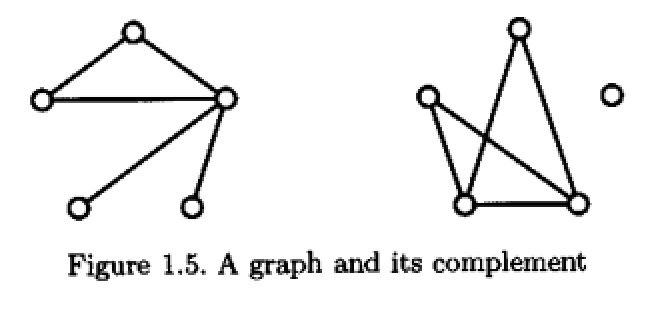
图$X$的补图$\overline X$是这样一个图: 它满足$V(X)=V(\overline X),$
但两顶点在$\overline X$中相邻当且仅当它们在$X$中不相邻.
容易证明如下引理:
引理 1.3. $\operatorname{Aut}(X)\cong \operatorname{Aut}(\overline X).$
若$X$是有向图, 那么对于同构, 我们要求它是保方向的.
同态
给两个图$X,Y,$ 映射$f:V(X)\rightarrow V(Y)$称为同态,
若$x\sim y\in X\Rightarrow f(x)\sim f(y)\in Y.$ 前面的同构当然也是同态.
图$X$为二分图, 若$V(X)$可划分为$V_1,V_2,$
使得每个边的端点分别在这两个集合中.
一个同态的例子是$V(X)\rightarrow V(K_2),$ 将$V_i$映到顶点$i$.
这一例子引申出图的染色问题. 一个图的正常染色(proper colouring),
指从$V(X)$到某有限(颜色)集的映射, 使得相邻的点映至不同的颜色.
如果$X$可由$k$种颜色正常染色, 称其可被$k-$染色.
称最小的$k$为图$X$的着色数(chromatic number), 记为$\chi(X).$
染上某种颜色的全体点构成独立集, 称为一个颜色类(colour class).
对于至少有一条边的二分图, 它的着色数即为$2.$
引理 1.4. $X$的着色数是最小的$r,$ 使得存在$X\rightarrow K_r$的同态.
证: 对同态$f:X\rightarrow Y,$ 易见对$y\in Y,$
$f^{-1}(y):=\{x\in V(X): f(x)=y\}$为独立集. 因此若有$X$到$K_r$的同态,
以$K_r$顶点为$r$个不同颜色, 对$X$中顶点按其像上色即可,
从而$\chi(X)\le r.$
若$\chi(X)$可被$r-$染色, 记颜色集为$\{1,\cdots,r\},$
将每个颜色类映到$K_r$中相应顶点即可. 因为$X$中相邻的点颜色不同,
而不同颜色在$K_r$中彼此相邻.
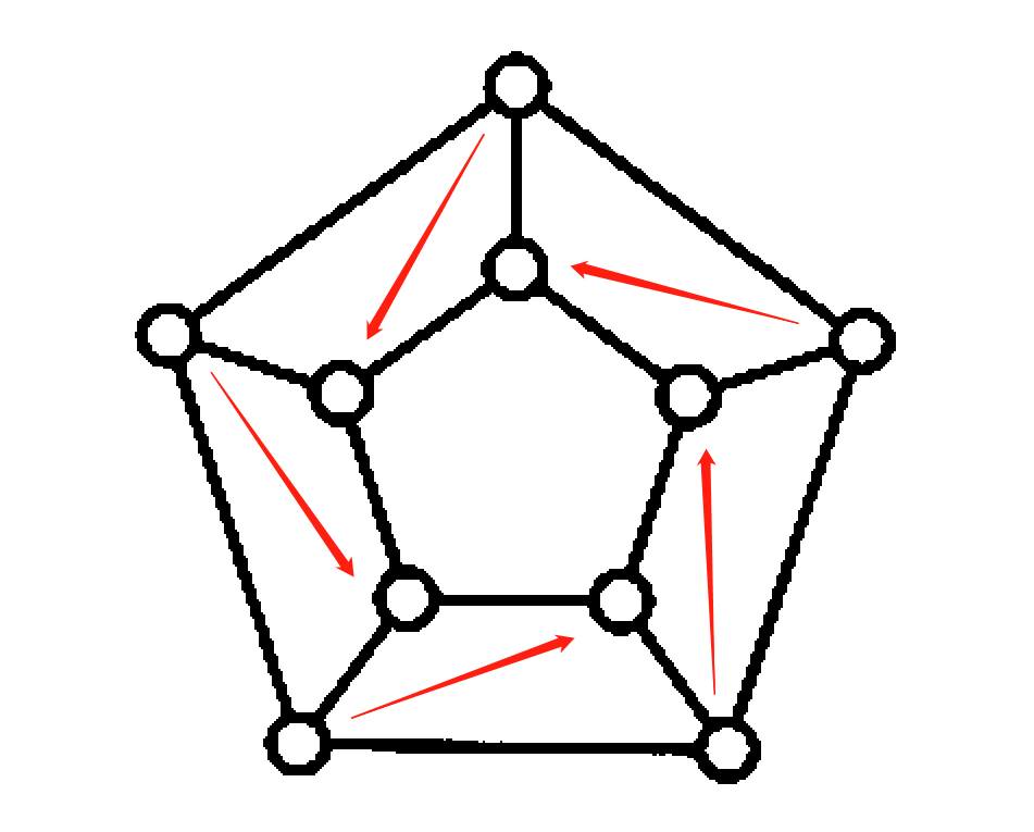
图$X$到其子图$Y$的同态$f$称为收缩, 若$f|_Y$为恒等映射.
此时称$Y$为$X$的收缩核. 如对如下的图, 按红色箭头所示构造同态,
则内侧的五边形成为原图的收缩核.
对有向图的同态, 只需将保相邻改为保有序对即可. 需要注意的是,
以上讨论均默认图中无环. 边称为圈(loop), 若其两端点是同一个点.
允许圈存在的图的同态的性质将大有不同.
一个例子是将任意顶点集映到有圈的点的映射都是同态.
图$X$到自身的同态称为自同态, 自同态全体构成幺半群. 自同构群包含在其中.
循环图
接下来介绍很重要的一类图, 称为循环图(circulant graph):
它是一个有向图$X=X(\mathbb{Z}_n,C),$
集合$C\subset \mathbb{Z}_n\setminus\{0\}.$ 其顶点为$\mathbb{Z}_n$中元素,
$(i,j)$为$X$中的弧当且仅当$j-i\in C.$
$X(\mathbb{Z}_n,C)$称为$n$阶循环图, 以$C$为连接集.
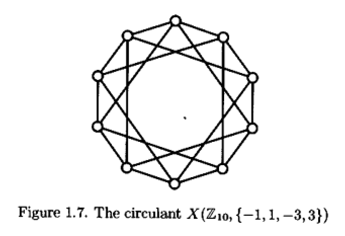
若$\,\forall\,c\in C,$ $-c\in C,$ 那么$(i,j)$为弧当且仅当$(j,i)$为弧,
从而$X$可以视为无向图. 易见前面提到的环即为$X(\mathbb{Z}_n,\{\pm 1\}),$
是循环图的一种, 记为$C_n$.
Johnson图
对正整数$v\ge k\ge i,$ 图$J(v,k,i)$是这样一个无向图:
设有含$v$个元素的集合$\Omega,$
图以$\Omega$中含$k$个元素的全体子集为顶点,
两点连边当且仅当其对应子集之交含$i$个元素. 因此它含$\binom{v}{k}$个顶点,
为正则图, 每点以$\binom{k}{i}\binom{v-k}{k-i}$为度.
引理 1.5. $J(v,k,i)\cong J(v,v-k,v-2k+i).$
证: 将每个含$k$元素子集映到它在$\Omega$中的补集即可.
易见两补集交集含$v-2k+i$个元素当且仅当原来的两集合含$i$个元素.
因此这样的映射是同构.
由该引理, 我们总是可默认$v\ge 2k.$ 这时称$J(v,k,k-1)$为Johnson图,
$J(v,k,0)$为Kneser图. 由于$\Omega$中元素的置换诱导子集间的置换,
我们有如下引理:
引理 1.6. $S_v\subset \operatorname{Aut}(J(v,k,i)).$
边图
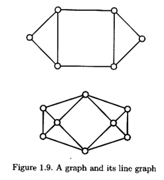
图$X$的边图(line graph)$L(X)$是这样一个图: 它以$X$的边为顶点,
两顶点连边当且仅当它们在$X$中对应的边有公共顶点.
星形图$K_{1,n}$为由$1$个顶点与其$n$个邻点构成的图.
它的边图即为完全图$K_n.$ 对于环$C_n,$ 它与其边图同构.
对每个边考虑其两个顶点, 有如下引理:
引理 1.7. 若$X$是$k-$正则图, 那么$L(X)$是$2k-2$正则的.
$X$中每个度为$k$的顶点都决定了$L(X)$中大小为$k$的团. 若$X$含$n$个顶点,
则$L(X)$中有对应的$n$个团, 使得$L(X)$的每个顶点最多在其中的两个团中,
每条边恰在其中一个团里. 事实上通过构造的方法, 有如下的逆命题:
定理 1.8 (Krausz). 非空图是某个图的边图当且仅当它的边集可以划分为若干个团, 使得每个顶点最多在其中两个团中.
若$X$不含三角形(大小为$3$的团), 则当$L(X)$中某个点有两邻点,
两邻点都在前面所述的某个团中时, 这个点也在该团中.
不然它们对应的边在$X$即构成三角形.
因此由$X$顶点决定的$L(X)$中的团都是极大的.
显然$X\cong Y\Rightarrow L(X)\cong L(Y),$ 但反过来不见得对,
比如$L(K_{1,3})\cong L(K_3).$
不过Whitney证明了事实上这是唯一一个连通情况下的反例.
我们来证明下面弱一点的命题.
引理 1.9. 若$X,Y$最小度大于$3,$ 则$X\cong Y\Leftrightarrow L(X)\cong L(Y).$
证: 只需注意到在边图中,
含三个点以下的团不见得还原为以某顶点出发星形图,
但三个点以上的团还原时必然还原为星形图. 只需说明四个边两两有公共顶点时,
一定是$K_{1,4}$的形状. 不然其中三个边还原时一定还原为三角形,
而这时无法再添加第四条边使得两两边有公共顶点.
从而在每个顶点度均大于$3$的情况下,
$n$个顶点对应的$n$个极大团大小大于$3,$
且反过来每个大小大于$3$的极大团都对应一个顶点.
从而顶点集到大小大于$3$的极大团全体间有一个双射,
且满足顶点相邻当且仅当对应的极大团有公共点.
因此图的属性与其边图属性互相决定,
故$X\cong Y\Leftrightarrow L(X)\cong L(Y).$
另一个关于边图的有趣描述是:
定理 1.10 (Beineke). 图是边图当且仅当它的每个最多含六个点的诱导子图是边图.
我们称二分图是半正则的, 若它有$2$-染色使得颜色相同的点度相同.
最简单的例子是完全二分图$K_{m,n},$
由两个含$m$个点与$n$个点的独立集构成, 其间两两连接.
引理 1.11. 若连通图$X$的边图$L(X)$为正则图, 则$X$是正则的, 或是半正则的二分图.
证: 设$L(X)$是$k-$正则的, 那么$X$中每对邻点的度之和恒为$k+2.$
因此连通的$X$中所有点的度最多只有两种取值. 若只有一种取值,
那么就是正则图; 如果有两种不同取值, 那么按这两种取值染色即可.
这样只有相异颜色的点度之和满足要求, 因此相同颜色的点必不相邻.
且这样染色后, 颜色相同的点度相同, 是半正则的.
可平面图
我们已经看到, 用图示来表示图很方便. 若图可被无交线地绘制出来,
则称其为可平面图(planar graph). 更精确地, 我们考虑将图映到平面上.
将顶点映至点, 边映至连接两点的连续无自交的曲线,
称这样的映射为平面嵌入, 若无公共点的边对应曲线不相交,
有公共顶点的边对应的曲线仅在平面上对应点相交.
图称为可平面的当且仅当存在这样一个平面嵌入.
平面图(plane graph)为取好平面嵌入的可平面图.
平面图的边将平面划分为若干区域, 称为平面图的面. 除了一个区域外,
其它区域都是有界的, 称这个无界的区域为无穷面或外面(external
face). 面的长度指框住它边的个数.
著名的欧拉公式给出平面图点线面的关系:
定理 1.12 (Euler). 若连通平面图有$n$个顶点, $e$条边与$f$个面, 那么$n-e+f=2.$
可平面图称为极大可平面图, 如果再添加一条边就不再是可平面的了.
如果可平面图的平面嵌入有长度大于$3$的面, 那么一定可以再添一条边.
因此极大可平面图的平面嵌入所有面长度均为$3$. 若每个点度至少是$2$,
则每条边恰在两个面中, 我们有$2e=3f,$ 从而$e=3n-6.$
事实上若含$n$个点的可平面图有$3n-6$条边, 它一定是极大的.
这样的图称为平面三角剖分.
一个图的平面嵌入有很多种, 这会导致平面图的面有所不同, 如下图所示.
一个很重要的拓扑结论是, $3-$连通的图本质上只有唯一一种嵌入方式.
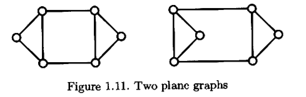
给定平面图$X,$ 我们可以生成对偶图(dual graph)$X^\ast,$
以$X$的面为$X^\ast$顶点, 对每条$X$中两面的公共边,
绘制一条(跨公共边的)$X^\ast$中的边连接两面对应的顶点.
注意$X^\ast$中可能有重边(multiple edge), 即两个点间连接多个边.
除了特殊说明, 我们默认不考虑图中出现重边的情况.
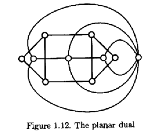
若图与其对偶图同构, 则称其自对偶(self-dual), 如完全图$K_4.$
对连通的图$X,$ 可以说明$X\cong (X^\ast)^\ast.$
嵌入的概念可以从平面推广到任意曲面上, 对偶也类似.
一个例子是非可平面图的完全图$K_6$可以嵌入到射影平面上,
是射影平面的一个三角剖分.
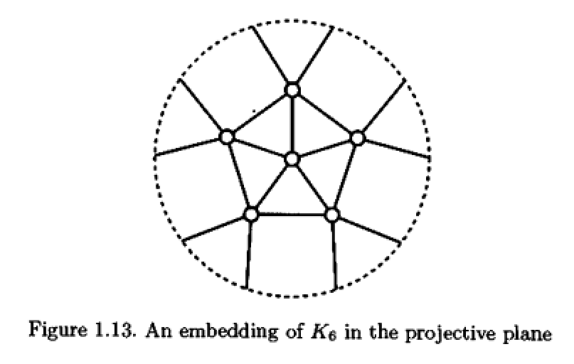
另一个例子是完全图$K_7$不是可平面图, 也不能嵌入到射影平面上,
但是可以嵌入到环面上.
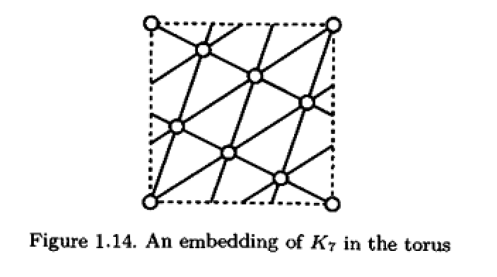
文章最后更新于 2021-09-16 14:51:40
Graphs
Figure $X$ is given by vertex set $V(X),$ Bianji $E(X)$Composition.
Each (undirected) edge is an unordered pair $\{x,y\},$, which is often represented by $xy$. If $xy\in E,$
Then it is called $x,y$ point adjacent, recorded as $x\sim y.$
If there is a bijection$\varphi: V(X)\rightarrow V(Y),$
Such that $V(X)$ is in $x\sim y$ if and only if $V(Y)$ is in $\varphi(x)\sim\varphi(y),$
Then we call the graphs $X$ and $Y$ isomorphism. When drawing representations, numbers are often used to label vertices.
Call the picture complete , if both its vertices are adjacent.
The complete graph with $n$ vertices is called $K_n.$. The graph is said to be empty of,
If the edge set is an empty set and has at least one vertex; the graph is said to be invalid(null) of,
If the edge set and the point set are both empty sets. These two concepts are proposed for narrative convenience.
The previous pictures are all simple diagram. Sometimes edge set $E(X)$ is replaced by directed edge set $A(X),$
called directed graph. At this time, the edges are ordered pairs, which are represented by arrows in the diagram and are called arc.
An undirected graph is sometimes also considered as a directed graph in which each undirected edge is two directed edges.
Generally, simple graphs are considered by default. The vertex set can actually have an infinite number of elements,
But this book considers by default finite graph.
subplot
If the graph $Y$ satisfies $V(X)\subset V(Y),$ $E(X)\subset E(Y),$
Then $Y$ is called $X$ subplot. If $V(Y)=V(X),$ is also satisfied, then $Y$ is called $X$. Generate subgraph.
If the vertices in subgraph $Y$ are adjacent if and only if they are adjacent in $X$, then $Y$ is called an induced subgraph of $X$.
It can be seen that the generated subgraph is obtained by deleting edges, while the induced subgraph is obtained by deleting points and their adjacent edges.
There are several important concepts related to subgraphs: If a subgraph is a complete graph, it is called a clique.
If the induced subgraph of a certain vertex set is empty, it is called independent set.
The size of the largest clique in graph $X$ is recorded as $\omega(X),$, and the size of the largest independent set is recorded as $\alpha(X).$.
These are two very important properties of graphs.
On the graph, the length from vertex $x$ to $y$ is $r$. road,
Refers to a sequence composed of $r+1$ different vertices, with $x$ as the head and $y$ as the tail.
And adjacent vertices in the sequence are also adjacent in the graph. If any two points on the graph have roads starting and ending with them,
Then the graph is said to be connected , otherwise it is disconnected.
The graph is disconnected, which is equivalent to dividing the vertex set of the graph $X$ into two sets $R,S,$.
So that the vertices in $R$ and the vertices in $S$ are not adjacent.
At this time we can say that the graph $X$ is the intersection-free union of the vertex sets $R$ and $S$ induced subgraphs. A maximum connected induced subgraph,
called graph $X$ connected component, abbreviated as branch.
one cycle Refers to a connected graph, each vertex has exactly two neighbors;
A ring in a graph refers to a ring that is a subgraph. It is easy to prove that if every point in the graph has at least two neighboring points,
Then the graph must contain a cycle. A connected acyclic graph is called tree,
The acyclic graph can be split into the non-intersecting union of several maximal connected acyclic graphs, so it is called forest.
If a generated subgraph is a tree, it is called spanning tree. It is easy to see that a graph has a spanning tree if and only if it is connected.
A maximal spanning forest refers to a spanning subgraph composed of spanning trees for each branch.
automorphism
The isomorphism of graph $X$ to itself is an automorphism. It is easy to prove that all automorphisms form a group,
Recorded as $\operatorname{Aut}(X).$
Obviously $\operatorname{Aut}(X)\subset \operatorname{Sym}(V(X)).$
The latter refers to the symmetric group, that is, all permutations of the set $V(X)$.
A basic example is $\operatorname{Aut}(K_n)\cong \operatorname{Sym}(V(K_n))=S_n.$
Generally speaking, it is not easy to determine whether two graphs are isomorphic, and whether a graph has non-trivial automorphism.
The image of $v$ under permutation $g$ is recorded as $v^g.$. When $g\in \operatorname{Aut}(X)$,
For subgraph $Y\subset X,$, the subgraph $Y^g\subset X.$ can be defined edge-preservingly.
$Y$ and $Y^g$ are naturally isomorphic.
Vertex$x$ Valency, refers to the number of neighbors of $x$. The maximum (minimum) degree of the graph $X$,
That is, it refers to the maximum (minimum) value of all vertex degrees. If the degree of each vertex of the graph is $k,$
is called $k-$Regular graph.
Lemma 1.1. If $x\in X,$ $g\in \operatorname{Aut}(X),$ then $x$ and $x^g$ have the same degree.
Certificate:
Just use the induced subgraph $N(x)$ of $x$ and all its neighbors to satisfy $N(x)\cong N(x)^g=N(x^g)$.
The two vertices $x,y$ in the graph $X$ distance $d_X(x,y),$ refers to the length of the shortest circuit connecting $x,y$.
If $X$ is clear, the distance can be abbreviated as $d(x,y).$. A simple lemma is as follows:
Lemma 1.2. $\,\forall\,x,y\in X,$ $g\in \operatorname{Aut}(X),$ $d(x,y)=d(x^g,y^g).$
Figure$X$ Complement the picture $\overline X$ is such a graph: It satisfies $V(X)=V(\overline X),$
But two vertices are adjacent in $\overline X$ if and only if they are not adjacent in $X$.
It is easy to prove the following lemma:
Lemma 1.3. $\operatorname{Aut}(X)\cong \operatorname{Aut}(\overline X).$
If $X$ is a directed graph, then for isomorphism, we require it to be direction-preserving.
homomorphism
Given two graphs $X,Y,$, the mapping $f:V(X)\rightarrow V(Y)$ is called homomorphism,
If $x\sim y\in X\Rightarrow f(x)\sim f(y)\in Y.$ the previous isomorphism is of course also a isomorphism.
Figure $X$ is bipartite graph, if $V(X)$ can be divided into $V_1,V_2,$
Such that the endpoints of each edge are in these two sets respectively.
An example of a homomorphism is $V(X)\rightarrow V(K_2),$ mapping $V_i$ to vertex $i$.
This example leads to the problem of graph coloring. A graph normal coloring,
It refers to the mapping from $V(X)$ to a certain finite (color) set, so that adjacent points are mapped to different colors.
If $X$ can be dyed normally by $k$ colors, it is said that it can be dyed by $k-$ Dyeing.
Call the smallest $k$ the graph $X$ chromatic number, recorded as $\chi(X).$
All points dyed with a certain color form an independent set, called a color class.
For a bipartite graph with at least one edge, its coloring number is $2.$
Lemma 1.4. The shading number of $X$ is the smallest $r,$ such that there is a homomorphism of $X\rightarrow K_r$.
Certificate: Pair homomorphism $f:X\rightarrow Y,$ Easy to see pair $y\in Y,$
$f^{-1}(y):=\{x\in V(X): f(x)=y\}$ is an independent set. Therefore, if there is a homomorphism from $X$ to $K_r$,
Use $K_r$ vertices as $r$ different colors, and color the vertices in $X$ according to their images.
Thus $\chi(X)\le r.$
If $\chi(X)$ can be dyed by $r-$, record the color set as $\{1,\cdots,r\},$
Just map each color class to the corresponding vertex in $K_r$. Because the adjacent points in $X$ have different colors,
And different colors are next to each other in $K_r$.
The homomorphism $f$ from graph $X$ to its subgraph $Y$ is called contraction, if $f|_Y$ is an identity mapping.
At this time, $Y$ is called the shrinking kernel of $X$. As shown in the figure below, construct the homomorphism as shown by the red arrow,
Then the five inner sides form the contraction core of the original image.
For the homomorphism of directed graphs, just change the preservation of adjacency to the preservation of ordered pairs. It should be noted that,
The above discussions all assume that there are no cycles in the graph. The edges are called loop, if its two endpoints are the same point.
The properties of homomorphisms of graphs that allow cycles will be quite different.
An example is that any mapping from a set of vertices to a point with a cycle is homomorphic.
The homomorphism of the graph $X$ to itself is called an automorphism, and all automorphisms constitute a monoid group. The automorphism group is included in it.
cycle diagram
Next, we introduce a very important type of graph, called circulant graph:
It is a directed graph $X=X(\mathbb{Z}_n,C),$
The vertices of the set $C\subset \mathbb{Z}_n\setminus\{0\}.$ are elements in $\mathbb{Z}_n$,
$(i,j)$ is an arc in $X$ if and only if $j-i\in C.$
$X(\mathbb{Z}_n,C)$ is called $n$ order cyclic graph, and $C$ is the connected set.
If $\,\forall\,c\in C,$ $-c\in C,$ then $(i,j)$ is an arc if and only if $(j,i)$ is an arc,
Therefore $X$ can be regarded as an undirected graph. It is easy to see that the ring mentioned above is $X(\mathbb{Z}_n,\{\pm 1\}),$
It is a type of cyclic graph, denoted as $C_n$.
Johnson diagram
The graph $J(v,k,i)$ of positive integers $v\ge k\ge i,$ is such an undirected graph:
Let there be a set $\Omega,$ containing $v$ elements.
The graph takes all subsets containing $k$ elements in $\Omega$ as vertices,
An edge is connected between two points if and only if the intersection of its corresponding subsets contains $i$ elements. Therefore, it contains $\binom{v}{k}$ vertices,
It is a regular graph, and each point has $\binom{k}{i}\binom{v-k}{k-i}$ as the degree.
Lemma 1.5. $J(v,k,i)\cong J(v,v-k,v-2k+i).$
Certificate: Just map each subset containing $k$ elements to its complement in $\Omega$.
It is easy to see that the intersection of two complementary sets contains $v-2k+i$ elements if and only if the original two sets contain $i$ elements.
Therefore such mappings are isomorphic.
According to this lemma, we can always default to $v\ge 2k.$. In this case, we call $J(v,k,k-1)$ Johnson diagram,
$J(v,k,0)$ is Kneser diagram. Since the permutation of elements in $\Omega$ induces permutation between subsets,
We have the following lemma:
Lemma 1.6. $S_v\subset \operatorname{Aut}(J(v,k,i)).$
side picture
Figure$X$ line graph $L(X)$ is such a graph: it has the edge of $X$ as its vertex,
Two vertices are connected by an edge if and only if their corresponding edges in $X$ have a common vertex.
star chart $K_{1,n}$ is a graph consisting of $1$ vertices and their $n$ neighbors.
Its edge graph is the complete graph $K_n.$ and for the ring $C_n,$ it is isomorphic to its edge graph.
Considering its two vertices for each edge, we have the following lemma:
Lemma 1.7. If $X$ is a $k-$ regular graph, then $L(X)$ is a $2k-2$ regular graph.
Each vertex with degree $k$ in $X$ determines a cluster with size $k$ in $L(X)$. If $X$ contains $n$ vertices,
Then there are corresponding $n$ clusters in $L(X)$, so that each vertex of $L(X)$ is in at most two of the clusters,
Each edge is in exactly one of the groups. In fact, through the construction method, there is the following inverse proposition:
Theorem 1.8 (Krausz). A non-empty graph is an edge graph of a graph if and only if its edge set can be divided into several cliques, such that each vertex is in at most two of the cliques.
If $X$ does not contain triangle (a group with size $3$), then when a point in $L(X)$ has two neighboring points,
When both adjacent points are in a certain group as mentioned above, this point is also in that group.
Otherwise, their corresponding sides form a triangle in $X$.
Therefore, the cliques in $L(X)$ determined by the vertices of $X$ are all maximal.
Obviously $X\cong Y\Rightarrow L(X)\cong L(Y),$ but the reverse is not necessarily true,
For example $L(K_{1,3})\cong L(K_3).$
However, Whitney proved that this is in fact the only counterexample in the connected case.
Let us prove the weaker proposition below.
Lemma 1.9. If the minimum degree of $X,Y$ is greater than $3,$, then $X\cong Y\Leftrightarrow L(X)\cong L(Y).$
Certificate: Just note that in the side plot,
A cluster containing less than three points may not necessarily be reduced to a star graph starting from a certain vertex.
However, when a group with more than three points is restored, it must be restored to a star graph. It only needs to be explained that when four sides have common vertices in pairs,
It must be the shape of $K_{1,4}$. Otherwise, three of the sides must be restored to a triangle when restored.
At this time, it is impossible to add a fourth edge so that both sides have common vertices.
Therefore, when the degree of each vertex is greater than $3$,
The size of the $n$ maximal cliques corresponding to $n$ vertices is greater than $3,$
And conversely, each maximal clique with a size larger than $3$ corresponds to a vertex.
Therefore, there is a bijection between the vertex set and the maximal group whose size is greater than $3$,
And the vertices are adjacent if and only if the corresponding maximal cliques have common points.
Therefore, the properties of the graph and its edge graph properties determine each other,
Therefore$X\cong Y\Leftrightarrow L(X)\cong L(Y).$
Another interesting description of edge graphs is:
Theorem 1.10 (Beineke). A graph is an edge graph if and only if its induced subgraphs each containing at most six points are edge graphs.
We call a bipartite graph a Semi-regular , if it has $2$-dying such that points with the same color have the same degree.
The simplest example is complete bipartite graph $K_{m,n},$
It consists of two independent sets containing $m$ points and $n$ points, connected in pairs.
Lemma 1.11. If the edge graph $L(X)$ of the connected graph $X$ is a regular graph, then $X$ is a regular or semi-regular bipartite graph.
Certificate: Assume $L(X)$ is regular $k-$, then the sum of the degrees of each pair of adjacent points in $X$ is always $k+2.$
Therefore, the degree of all points in connected $X$ can only take on two values at most. If there is only one value,
Then it is a regular graph; if there are two different values, then just dye it according to these two values.
In this way, only the sum of point degrees of different colors meets the requirements, so points of the same color must not be adjacent.
And after dyeing in this way, points with the same color have the same degree, which is semi-regular.
Available floor plan
We have seen that it is convenient to represent graphs graphically. If the graph can be drawn without intersecting lines,
is called planar graph.More precisely, we consider mapping the graph onto a plane.
Map vertices to points and edges to continuous curves connecting two points without self-intersection,
Call such a mapping planar embedding, if the curves corresponding to the edges without common points do not intersect,
Curves corresponding to edges with common vertices only intersect at corresponding points on the plane.
The graph is called Planar iff there exists such a planar embedding.
plane graph A planar graph embedded in order to obtain a good plane.
The edges of a plane diagram divide the plane into several areas, which are called the sides of the plane diagram. noodles.Except for one area,
All other areas are bounded, and this unbounded area is called infinite surface or external
face).The length of a face refers to the number of sides that frame it.
The famous Euler formula gives the relationship between points, lines and surfaces in a plane diagram:
Theorem 1.12 (Euler). If the connected plane graph has $n$ vertices, $e$ edges and $f$ faces, then $n-e+f=2.$
The plan view can be called Great floor plan, if one more edge is added, it is no longer planar.
If the plane of a planar graph is embedded with a face whose length is greater than $3$, then you can definitely add another edge.
Therefore, the length of all faces embedded in the plane of a maximally planar graph is $3$. If the degree of each point is at least $2$,
Then each edge lies exactly in two faces, we have $2e=3f,$ and thus $e=3n-6.$
In fact, if a planar graph containing $n$ points has $3n-6$ edges, it must be maximal.
Such a graph is called Plane triangulation.
There are many kinds of planar embeddings for a graph, which will cause the faces of the planar graph to be different, as shown in the figure below.
A very important topological conclusion is that $3-$ connected graphs essentially have only one embedding method.
Given a floor plan $X,$ we can generate dual graph $X^\ast,$
Taking the face of $X$ as the vertex of $X^\ast$, for each common edge of the two faces in $X$,
Draw an edge in $X^\ast$ (across a common edge) connecting the corresponding vertices on both sides.
Note that $X^\ast$ may contain Multiple edges, that is, multiple edges are connected between two points.
Unless otherwise specified, we do not consider duplicate edges in the graph by default.
If a graph is isomorphic to its dual graph, it is called self-dual, such as the complete graph $K_4.$
For the connected graph $X,$, it can be explained $X\cong (X^\ast)^\ast.$
The concept of embedding can be generalized from the plane to any surface, and the duality is similar.
An example is that a complete graph $K_6$ of a non-planar graph can be embedded on a projective plane,
is a triangulation of the projective plane.
Another example is that the complete graph $K_7$ is not planar and cannot be embedded in the projective plane.
But it can be embedded on the torus.
The article was last updated on 2021-09-16 14:51:40