Machine-translated from Chinese.
介绍
现在开始我们对空间形式, 即常截面曲率的完备黎曼流形进行研究.
我们有如下基本结果:
定理 1. $\,\forall\,c\in \mathbb{R},$ $n\in \mathbb{Z}_+,$ $\,\exists\,$等距变换下唯一的常截面曲率$c$的单连通$n$维空间形式.
定理完整证明于下章给出, 本节我们注重于存在性部分. 设有黎曼度量$g,$
截面曲率为$K,$ 那么对于正常数$A,$ 度量$Ag$的截面曲率为$\frac{1}{A}K.$
因此我们只需考虑截面曲率为$0,\pm 1$的空间形式. 对于$c=0,$
取$\mathbb{R}^n$即可; 对于$c=1,$ 取熟知的单位球面$S^n$即可; 对于$c=-1,$
需要取配备双曲度量, 即
$$
g=\frac{4}{\left(1-\sum_i \left(x^i\right)^2\right)^2}\sum_i dx^i\otimes dx^i
$$
的单位球$B^n.$ 我们引入新的概念后来说明后两个结论.
全测地子流形
定义
设$M$为黎曼流形$\overline{M}$的子流形, 配备诱导度量.
若$\overline{M}$中任一与$M$相切的测地线全部位于$M$中,
则称$M$是$\overline{M}$中的全测地子流形. 可以看出,
全测地子流形是十分稀少的, 几乎所有黎曼流形都没有任何全测地子流形.
不过由此可以引入一个新的几何量, 这是十分有意义的.
引理 2. $M$是$\overline{M}$的全测地子流形的充要条件是, 对$M$中任何向量场$X,Y,$ $D_XY=\overline{D}_XY,$ 这里$D,\overline{D}$分别为$M,\overline{M}$上的Levi-Civita联络.
证: 首先设$M$是$\overline{M}$的任一子流形. 对$M$中向量场$X,Y,$ 定义
$$
S(X,Y):=D_XY-\overline{D}_XY,
$$
$S(X,Y)$是$\overline{M}$中仅定义在$M$上的向量场. 此时,
对$M$上任意函数$f,$
$$
S(fX,Y)=fS(X,Y)=S(X,fY).
$$
因此可定义$S:M_x\otimes M_x\rightarrow \overline{M}_x,$
$$
S(v,w)=S(V,W),\quad \,\forall\,V(x)=v,W(x)=w\in M_x,
$$
$V,W$为$M$中任意满足上述条件的向量场. 由Levi-Civita联络的对称性可知,
$$
S(v,w)=S(w,v).
$$
现设$M$为$\overline{M}$的全测地子流形, 断言:
$$
S(v,v)=0,\quad \,\forall\,v\in M_x, x\in M.
$$
设$\gamma$为$\overline{M}$中以$v$为初始切向量的测地线,
$\overline{D}_{\dot\gamma}\dot\gamma=0,$ 则$\gamma$也是$M$中测地线,
$D_{\dot\gamma}\dot\gamma=0.$ 因此
$$
S(v,v)=D_{\dot\gamma(0)}\dot\gamma-\overline{D}_{\dot\gamma(0)}\dot\gamma=0.
$$
从而,
$$
S(v+w,v+w)=2S(v,w)=0\,\Rightarrow\, D_XY=\overline{D}_XY,\quad \,\forall\,X,Y\in \mathfrak{X}(M).
$$
反之, 设$S\equiv 0.$ 取$\overline{M}$中与$M$相切的测地线$\gamma,$
欲说明$\gamma\subset M.$ 取$M$中测地线$\xi,$ 与$\gamma$初始切向量相同.
此时,
$$
\overline{D}_{\dot\xi}\dot\xi=D_{\dot\xi}\dot\xi\equiv 0,
$$
因此$\xi$也是$\overline{M}$中测地线. 由唯一性即知$\xi=\gamma,$
从而$\gamma$确实落在$M$中.
注 3. 上述$S$称为$M$在$\overline{M}$中的第二基本形式, 关于它的讨论将在后续章节提到.
由于曲率张量由Levi-Civita联络定义, 我们有如下推论:
引理 4. 设$M$是$\overline{M}$的一个全测地子流形, $K,\overline{K}$分别为$M,\overline{M}$的截面曲率函数, 则$\,\forall\,x\in M,$ 对于任意$2$-平面$\Pi\subset M_x,$ $K(\Pi)=\overline{K}(\Pi).$
等距变换
我们先看一个例子, 设$\gamma$为弧长参数曲线,
且存在等距变换$\varphi$以$\gamma$为固定点集.
那么断言$\gamma$为正规测地线. $\,\forall\,t,$
取$\xi$为以$\dot{\gamma}(t)$为初始切向量的测地线,
那么由于等距变换保持局部极短性质, $\varphi(\xi)$也是测地线,
且以$d\varphi (\dot\gamma(t))=\dot\gamma(t)$为初始切向量.
由唯一性知$\varphi(\xi)=\xi,$ $\xi$轨迹为固定点集,
从而$\gamma$与$\xi$在公共定义域上相同, 为正规测地线. 更一般地,
我们有如下结论:
引理 5. 一个等距变换的固定点集为全测地子流形(不一定连通).
证:
只需集中证明$\overline{M}$关于等距变换$\varphi$的固定点集$M$的确是一个子流形,
其后的说明与前面的讨论一致. 定义
$$
\mathscr{F}:=\{v\in \overline{M}_x:d\varphi(v)=v\},
$$
只需说明$\exp_x(\mathscr{F}\cap B(\delta))=M\cap B_\delta,$
其中$\delta$充分小使$\exp_x$在球上是微分同胚.
这样就建立了$M$上的坐标邻域, 使之成为子流形. 关于这一点的证明,
同样注意利用等距变换保持测地性, 以及测地线的唯一性即可.
空间形式
单位球面
引理 6. 单位球面$S^n$具常截面曲率$+1,$ $\,\forall\,n\ge 2.$
证: $n=2$时, $S^2$截面曲率即高斯曲率, 熟知为$+1.$ 对$n\ge 3,$
记$x\in \mathbb{R}^3,$ $y\in \mathbb{R}^{n-2},$
$\mathbb{R}^{n+1}$上的等距变换$\widetilde\varphi:(x,y)=(x,-y)$诱导了$S^n$上的等距变换$\varphi,$
以$\{(x,0)\}=S^2$为固定点集. 因此$S^2$是一个全测地子流形, 由引理,
$S^n$中与该$S^2$相切平面的截面曲率与$S^2$截面曲率相同, 为$+1.$
而对于$S^n,$ 任意两点处任意两个二维切平面间存在一个等距变换,
因此它是以$+1$为常截面曲率的空间形式.
双曲度量
引理 7. 配备双曲度量的单位球$B^n$是常截面曲率为$-1$的完备黎曼流形.
证: 首先讨论完备性. 由Hopf-Rinow定理,
我们可以证明从原点出发的测地线总可无限延伸,
进而$\exp_O$定义在整个切空间上, 从而流形是完备的.
考虑曲线$\xi(s)=\left(\frac{e^s-1}{e^s+1},0,\cdots,0\right).$
计算得到$s$为弧长参数,
且$\xi$为等距变换$(x^1,x^2,\cdots,x^n)\mapsto (x^1,-x^2,\cdots,-x^n)$的不动点集,
故$\xi$是测地线. 进而由对称性, 沿各个方向出发的测地线均可无限延伸.
接下来, 取$B^n$在$p$点的任一切平面$\Pi\subset \mathbb{R}^n,$
取$E$为包含$\Pi,p$的任一$3$维子空间. 由对称性, 不妨假设$E=\mathbb{R}^3,$
那么$E\cap B^n=B^3$是等距变换$(x^1,x^2,x^3,x^4,\cdots,x^n)\mapsto (x^1,x^2,x^3,-x^4,\cdots,-x^n)$的不动点集,
为全测地子流形. 因此只需证明$B^3$在诱导双曲度量下具常截面曲率$-1$即可.
为此采用球坐标计算即可. $n=2$的情形直接采用极坐标计算即可.
后面我们将配备双曲度量的单位球记作$H^n.$
测地线性质
接下来我们在空间形式中考虑测地线的性质. 直观来看,
考虑从一点出发的固定初始切向量夹角的两条测地线,
若以$\mathbb{R}^n$为基准, $S^n$的相比之下要靠拢, 而$H^n$的要发散.
这是截面曲率与测地线间的重要联系. 接下来我们取$n=2$来严格表述这一点.
注意由于$n=2$的情形为各自一般情形的全测地子流形,
对一般的$n$性质也是成立的.
现设$M=\mathbb{R}^2,S^2,H^2,$ 选定参考点$O\in M,$
定义半径为$r$的测地圆周:
$$
C(r)=\{x\in M,d(0,x)=r\}.
$$
当$r$充分小时,
$C(r)$即为$M_O$中半径为$r$的圆周在微分同胚$\exp_O$下的像.
它的长度就衡量了$M$上从$O$点出发测地线的散开率.
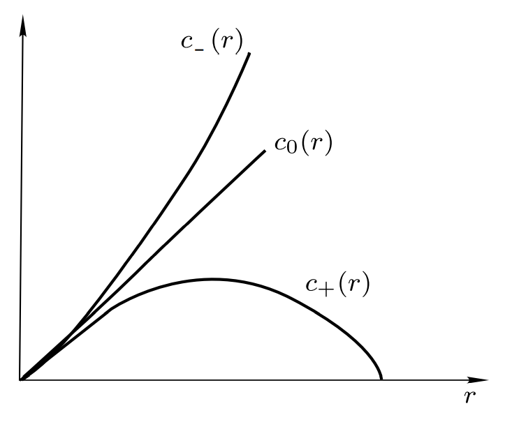
设$c_0(r),c_+(r),c_-(r)$分别是$\mathbb{R}^2,S^2,H^2$中$C(r)$的长度.
显然$c_0(r)=2\pi r,$ $c_+(r)=2\pi \sin r.$
最后计算可得$c_-(r)=2\pi \sinh r.$
它们都是齐性空间($H^n$的齐性将在后面说明),
因此参考点$O$选取不影响$C(r)$长度. 由图像立即可见负曲率将测地线推开,
而正曲率将测地线汇拢.
对任意完备二维黎曼流形$M,$ 选定参考点$O\in M,$
我们也来考虑测地圆周$C(r)$的长度$c(r).$ 令$r$充分小, 则
$$
c(r)=\int_0^{2\pi}\left|d\exp_O\left(\frac{d {} }{d {}\theta}(r,\theta)\right)\right|d\theta.
$$
可以看出我们不需要特别考虑$d\exp$对径向方向的影响.
我们先转而研究另一个对象, 之后再回来继续讨论这个问题.
Jacobi场
所谓$C^\infty$矩阵映射,
是指光滑映射$\gamma:[a,b]\times [c,d]\rightarrow M.$
可由此定义两个沿$\gamma$的向量场$T,U:$
$$
T(\gamma(t,u)):=d\gamma\left(\frac{\partial {} }{\partial {}t}(t,u)\right),\quad U(\gamma(t,u)):=d\gamma\left(\frac{\partial {} }{\partial {}u}(t,u)\right).
$$
每一个$u\in[c,d]$确定了一条曲线$\gamma_u(t)=\gamma(t,u).$
当$0\in[c,d]$时, 称$\gamma_0$为$C^\infty$矩形$\gamma$的基曲线.
若再假设每一条$\gamma_u$是$M$的测地线,
则称矩阵映射$\gamma$是单参数测地线族$\{\gamma_u\}.$ 于是我们有
$$
[T,U]=d\gamma\left(\left[\frac{\partial {} }{\partial {}t},\frac{\partial {} }{\partial {}u}\right]\right)=0,\quad D_TT=0.
$$
进而,
$$
D_TD_TU=D_TD_UT=D_TD_UT-D_UD_TT-D_{[T,U]}T=-R_{TU}T.
$$
限制在基曲线上, 我们就得到了:
$$
\ddot{U}+R_{\dot{\gamma}_0U}\dot{\gamma}_0=0.
$$
称上式为Jacobi方程, 称沿曲线$\gamma_0,$
符合上式的向量场$U$为Jacobi场.
称向量场$U$为$\{\gamma_u\}$的横截向量场, 于是得到:
引理 8. 单参数测地线族的横截向量场沿基曲线是一个Jacobi场.
反过来,
后面我们将说明沿测地线的每个Jacobi场都是某个单参数测地线族的横截向量场.
下面我们重新回到原来的讨论.
我们说明$d\exp_O\left(\frac{d {} }{d {}\theta}\right)$是某个单参数测地线族的横截向量场,
从而Jacobi方程就给出了曲率与$d\exp_O\left(\frac{d {} }{d {}\theta}\right)$之间决定性的联系,
也就可以看出曲率和$c(r)$之间的重要关系.
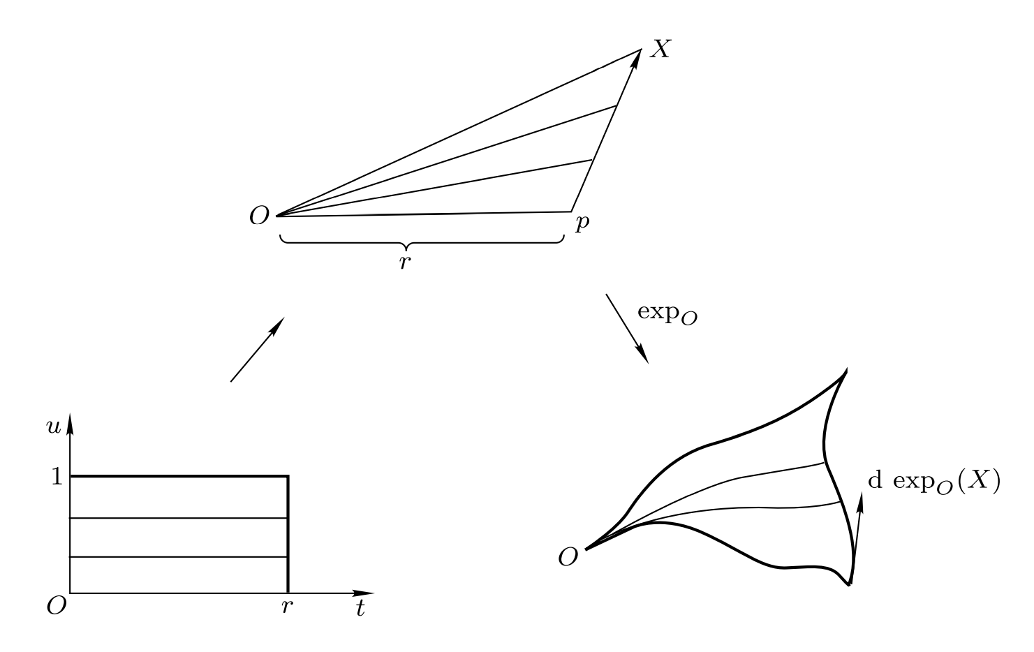
设$p\in M_O,$ $X$为$M_O$中向量,
那么$\Gamma(t,u):=\exp_O\frac{t}{r}(p+uX)$就定义了一个单参数测地线族,
$r=|p|,$ 满足
$$
U(0)=0,\quad \dot{U}(0)=\frac{1}{r}X.
$$
为证明第二个式子, 引入由$\exp_O:B(\delta)\approx B_\delta$决定的坐标系,
称为法坐标系, 满足:
$$
\left\{\begin{aligned}
&\left<{}\frac{\partial {} }{\partial {}x^i}(0),\frac{\partial {} }{\partial {}x^j}(0)\right>=\delta_{ij},&\,\forall\,i,j,\\
&D_{\frac{\partial {} }{\partial {}x^i}(0)}\frac{\partial {} }{\partial {}x^j}=0,&\,\forall\,i,j.
\end{aligned}\right.
$$
一式显然. 对于二式, 定义$\beta:M_O\times M_O\rightarrow \mathbb{R},$
$\beta(e_i,e_j)=D_{\frac{\partial {} }{\partial {}x^i}(0)}\frac{\partial {} }{\partial {}x^j},$
做线性延拓成为一个对称双线性型. 由于法坐标系下径向直线都是测地线,
$\beta(v,v)=0,$ 从而$\beta\equiv 0,$ 这就得到了第二式, 因此在法坐标系下,
$\Gamma_{ij}^k\equiv 0.$
现在就可以回来说明$\dot{U}(0)=\frac{1}{r}X.$ 由于$X$为常向量,
$\Gamma_{ij}^k\equiv 0,$
$$
D_{\dot{\gamma}_0(0)}U=\frac{1}{r}X+\frac{t}{r}D_{\dot{\gamma}_0(0)}X=\frac{1}{r}X.
$$
现取$X=\frac{d {} }{d {}\theta}(r,\theta)$就说明了$d\exp_O\left(\frac{d {} }{d {}\theta}\right)$确为某个单参数测地线族的横截向量场.
设$\gamma$是基曲线$\Gamma_0,$ $W(t)$为沿$\gamma$的单位平行向量场,
$W(t)\perp\dot{\gamma}(t).$ 对于横截向量场$U,$ 由Gauss引理,
它也与$\dot{\gamma}(t)$正交. 因此$U(t)=f(t)W(t).$ 由Jacobi方程,
$$
\ddot{f}+Kf=0,\quad f(0)=0,\quad \dot{f}(0)=1. \tag*{(\ast )}
$$
这里$K(t)$为$\gamma(t)$处的Gauss曲率.
应用到二维空间形式上, 我们就得到了:
$$
f(r)=\left\{\begin{aligned}
&r, &&K=0,\\
&\sin r, &&K=+1,\\
&\sinh r, &&K=-1.
\end{aligned}\right.
$$
这就是先前所求的$c_0,c_+,c_-.$
$(\ast )$式由Jacobi发现, 称其中的初始条件为标准的初始条件.
由于曲率控制测地线的性质,
可以预想到充分正曲率的流形应当是紧的(Bonnet-Myers定理),
而负曲率流形让我们期望一点处的指数映射将是一个微分同胚(Cartan-Hadamard定理).
最后给出一些评注. 假设$\dim M\ge 3,$ 称$M$是逐点常截面曲率的,
若$M$上每点所有$2$-平面的截面曲率相同. 经典的Schur定理表示,
流形是逐点常截面曲率的当且仅当它是常截面曲率的.
证明利用了第二Bianchi恒等式.
本节只讨论了单连通的空间形式. 其它的空间形式从几何, 群论,
拓扑等观点考虑也都是很重要的. 它们的分类工作也是一个重要的课题.
文章最后更新于 2022-04-19 14:01:46
Introduction
Now let's start with spatial form, that is Complete Riemannian manifold with constant cross-section curvature Conduct research.
We have the following basic results:
Theorem 1. $\,\forall\,c\in \mathbb{R},$ $n\in \mathbb{Z}_+,$ $\,\exists\,$ The only simply connected $n$ dimensional space form of constant cross-section curvature $c$ under isometric transformation.
The complete proof of the theorem is given in the next chapter. In this section we focus on the existence part. Let the Riemannian metric $g,$
The cross-sectional curvature is $K,$, then the cross-sectional curvature of the positive constant $A,$ metric $Ag$ is $\frac{1}{A}K.$
Therefore we only need to consider the spatial form with a cross-sectional curvature of $0,\pm 1$. For $c=0,$
Just take $\mathbb{R}^n$; for $c=1,$, just take the well-known unit sphere $S^n$; for $c=-1,$
Need to pick up equipment hyperbolic metric, that is
$$
g=\frac{4}{\left(1-\sum_i \left(x^i\right)^2\right)^2}\sum_i dx^i\otimes dx^i
$$
The unit ball $B^n.$ of we introduce new concepts and explain the last two conclusions later.
Full geodesic submanifold
definition
Let $M$ be the submanifold of the Riemannian manifold $\overline{M}$, equipped with induced metric.
If any geodesic in $\overline{M}$ that is tangent to $M$ is all located in $M$,
Then $M$ is said to be the total geodesic submanifold in $\overline{M}$. It can be seen that,
Fully geodesic submanifolds are very rare, and almost all Riemannian manifolds do not have any fully geodesic submanifolds.
However, a new geometric quantity can be introduced, which is very meaningful.
Lemma 2. The necessary and sufficient condition that $M$ is a full geodesic submanifold of $\overline{M}$ is that for any vector field $X,Y,$ $D_XY=\overline{D}_XY,$ in $M$, $D,\overline{D}$ is the Levi-Civita connection on $M,\overline{M}$ respectively.
Certificate: First, let $M$ be any submanifold of $\overline{M}$. Define the vector field $X,Y,$ in $M$
$$
S(X,Y):=D_XY-\overline{D}_XY,
$$
$S(X,Y)$ is the vector field in $\overline{M}$ only defined on $M$. At this time,
For any function $f,$ on $M$
$$
S(fX,Y)=fS(X,Y)=S(X,fY).
$$
Therefore $S:M_x\otimes M_x\rightarrow \overline{M}_x,$ can be defined
$$
S(v,w)=S(V,W),\quad \,\forall\,V(x)=v,W(x)=w\in M_x,
$$
$V,W$ is any vector field in $M$ that satisfies the above conditions. According to the symmetry of the Levi-Civita connection,
$$
S(v,w)=S(w,v).
$$
Now suppose $M$ is the total geodesic submanifold of $\overline{M}$, assert:
$$
S(v,v)=0,\quad \,\forall\,v\in M_x, x\in M.
$$
Let $\gamma$ be the geodesic in $\overline{M}$ with $v$ as the initial tangent vector,
$\overline{D}_{\dot\gamma}\dot\gamma=0,$ then $\gamma$ is also the geodesic in $M$,
$D_{\dot\gamma}\dot\gamma=0.$ Therefore
$$
S(v,v)=D_{\dot\gamma(0)}\dot\gamma-\overline{D}_{\dot\gamma(0)}\dot\gamma=0.
$$
Thus,
$$
S(v+w,v+w)=2S(v,w)=0\,\Rightarrow\, D_XY=\overline{D}_XY,\quad \,\forall\,X,Y\in \mathfrak{X}(M).
$$
On the contrary, let $S\equiv 0.$ take the geodesic $\gamma,$ in $\overline{M}$ that is tangent to $M$
To illustrate $\gamma\subset M.$, take the geodesic $\xi,$ in $M$ to be the same as the initial tangent vector of $\gamma$.
At this time,
$$
\overline{D}_{\dot\xi}\dot\xi=D_{\dot\xi}\dot\xi\equiv 0,
$$
Therefore $\xi$ is also a geodesic in $\overline{M}$. From the uniqueness, we know $\xi=\gamma,$
Thus $\gamma$ does fall within $M$.
Note 3. The above $S$ is called $M$ in $\overline{M}$ Second Fundamental Form, the discussion about it will be mentioned in subsequent chapters.
Since the curvature tensor is defined by the Levi-Civita connection, we have the following inference:
Lemma 4. Assume $M$ is a fully geodesic submanifold of $\overline{M}$, $K,\overline{K}$ is the cross-sectional curvature function of $M,\overline{M}$, then $\,\forall\,x\in M,$ for any $2$-plane $\Pi\subset M_x,$ $K(\Pi)=\overline{K}(\Pi).$
Isometric transformation
Let’s look at an example first. Let $\gamma$ be the arc length parameter curve,
And there is an isometric transformation $\varphi$ with $\gamma$ as the fixed point set.
Then assert $\gamma$ as a normal geodesic. $\,\forall\,t,$
Take $\xi$ as the geodesic with $\dot{\gamma}(t)$ as the initial tangent vector,
Then, since the isometric transformation maintains the local minimal property, $\varphi(\xi)$ is also a geodesic,
And take $d\varphi (\dot\gamma(t))=\dot\gamma(t)$ as the initial tangent vector.
From the uniqueness, we know that the trajectory $\varphi(\xi)=\xi,$ $\xi$ is a fixed point set,
Therefore, $\gamma$ and $\xi$ are the same in the common domain and are normal geodesics. More generally,
We have the following conclusions:
Lemma 5. An isometrically transformed set of fixed points is a fully geodesic submanifold (not necessarily connected).
Certificate:
We only need to focus on proving that $\overline{M}$ is indeed a submanifold with respect to the fixed point set $M$ of the isometric transformation $\varphi$,
The instructions that follow are consistent with the previous discussion. Definition
$$
\mathscr{F}:=\{v\in \overline{M}_x:d\varphi(v)=v\},
$$
Just explain $\exp_x(\mathscr{F}\cap B(\delta))=M\cap B_\delta,$
Among them, $\delta$ is a diffeomorphism on the sphere such that $\exp_x$ is a sufficient enlargement.
In this way, the coordinate neighborhood on $M$ is established, making it a submanifold. The proof of this point is,
Also pay attention to using isometric transformation to maintain geodesics and the uniqueness of geodesics.
spatial form
unit sphere
Lemma 6. The unit sphere $S^n$ has constant cross-sectional curvature $+1,$ $\,\forall\,n\ge 2.$
Certificate: When $n=2$, the cross-section curvature of $S^2$ is Gaussian curvature, which is known as $+1.$ versus $n\ge 3,$
Note $x\in \mathbb{R}^3,$ $y\in \mathbb{R}^{n-2},$
The isometric transformation $\widetilde\varphi:(x,y)=(x,-y)$ on $\mathbb{R}^{n+1}$ induces the isometric transformation $\varphi,$ on $S^n$
Let $\{(x,0)\}=S^2$ be the fixed point set. Therefore $S^2$ is a fully geodesic submanifold. According to the lemma,
The cross-sectional curvature of the plane tangent to $S^2$ in $S^n$ is the same as the cross-sectional curvature of $S^2$, which is $+1.$
For $S^n,$, there is an isometric transformation between any two two-dimensional tangent planes at any two points,
Therefore, it is a spatial form with $+1$ as the constant cross-section curvature.
hyperbolic metric
Lemma 7. The unit sphere $B^n$ equipped with a hyperbolic metric is a complete Riemannian manifold with constant cross-section curvature $-1$.
Certificate: First discuss the completeness. According to the Hopf-Rinow theorem,
We can prove that a geodesic starting from the origin can always extend infinitely,
Furthermore, $\exp_O$ is defined on the entire tangent space, so the manifold is complete.
Consider curve $\xi(s)=\left(\frac{e^s-1}{e^s+1},0,\cdots,0\right).$
The calculated $s$ is the arc length parameter,
And $\xi$ is the fixed point set of isometric transformation $(x^1,x^2,\cdots,x^n)\mapsto (x^1,-x^2,\cdots,-x^n)$,
Therefore $\xi$ is a geodesic. Furthermore, due to symmetry, geodesics starting in all directions can be extended infinitely.
Next, take any tangent plane $\Pi\subset \mathbb{R}^n,$ of $B^n$ at point $p$
Take $E$ as any $3$-dimensional subspace containing $\Pi,p$. Due to symmetry, we might as well assume that $E=\mathbb{R}^3,$
Then $E\cap B^n=B^3$ is the fixed point set of isometric transformation $(x^1,x^2,x^3,x^4,\cdots,x^n)\mapsto (x^1,x^2,x^3,-x^4,\cdots,-x^n)$,
is a fully geodesic submanifold. Therefore, it is only necessary to prove that $B^3$ has constant cross-section curvature $-1$ under the induced hyperbolic metric.
For this purpose, spherical coordinates can be used for calculation. In the case of $n=2$, polar coordinates can be used for calculation.
Later we will refer to the unit ball equipped with a hyperbolic metric as $H^n.$
Geodesic properties
Next we consider the properties of geodesics in spatial form. Intuitively,
Consider two geodesics starting from a point with a fixed initial tangent vector angle,
If $\mathbb{R}^n$ is used as the benchmark, $S^n$ will be closer in comparison, while $H^n$ will diverge.
This is an important connection between section curvature and geodesic. Next we take $n=2$ to strictly express this point.
Note that since the case $n=2$ is the full geodesic submanifold of the respective general case,
It is also true for the general $n$ property.
Now set $M=\mathbb{R}^2,S^2,H^2,$ and select the reference point $O\in M,$
Define a geodesic circle with radius $r$:
$$
C(r)=\{x\in M,d(0,x)=r\}.
$$
When $r$ is sufficiently small,
$C(r)$ is the image of the circle with radius $r$ in $M_O$ under diffeomorphism $\exp_O$.
Its length measures the spread rate of the geodesics on $M$ starting from the point $O$.
Let $c_0(r),c_+(r),c_-(r)$ be the length of $C(r)$ in $\mathbb{R}^2,S^2,H^2$ respectively.
Obviously $c_0(r)=2\pi r,$ $c_+(r)=2\pi \sin r.$
The final calculation can be $c_-(r)=2\pi \sinh r.$
They are all homogeneous spaces (the homogeneity of $H^n$ will be explained later),
Therefore, the selection of reference point $O$ does not affect the length of $C(r)$. It can be immediately seen from the image that the negative curvature pushes the geodesic apart.
And positive curvature brings geodesics together.
Select the reference point $O\in M,$ for any complete two-dimensional Riemannian manifold $M,$
Let us also consider the length $c(r).$ of the geodesic circle $C(r)$. Let $r$ be sufficiently small, then
$$
c(r)=\int_0^{2\pi}\left|d\exp_O\left(\frac{d {} }{d {}\theta}(r,\theta)\right)\right|d\theta.
$$
It can be seen that we do not need to specifically consider the influence of $d\exp$ on the radial direction.
Let's turn to another object first and come back to this issue later.
Jacobi field
So-called $C^\infty$ matrix mapping,
refers to smooth mapping $\gamma:[a,b]\times [c,d]\rightarrow M.$
From this we can define two along $\gamma$ vector field $T,U:$
$$
T(\gamma(t,u)):=d\gamma\left(\frac{\partial {} }{\partial {}t}(t,u)\right),\quad U(\gamma(t,u)):=d\gamma\left(\frac{\partial {} }{\partial {}u}(t,u)\right).
$$
Each $u\in[c,d]$ determines a curve $\gamma_u(t)=\gamma(t,u).$
When $0\in[c,d]$, $\gamma_0$ is called the base curve of $C^\infty$ rectangle $\gamma$.
If we further assume that each $\gamma_u$ is a geodesic of $M$,
Then it is said that matrix mapping $\gamma$ is Single parameter geodesic family $\{\gamma_u\}.$ So we have
$$
[T,U]=d\gamma\left(\left[\frac{\partial {} }{\partial {}t},\frac{\partial {} }{\partial {}u}\right]\right)=0,\quad D_TT=0.
$$
Furthermore,
$$
D_TD_TU=D_TD_UT=D_TD_UT-D_UD_TT-D_{[T,U]}T=-R_{TU}T.
$$
Restricted to the base curve, we get:
$$
\ddot{U}+R_{\dot{\gamma}_0U}\dot{\gamma}_0=0.
$$
Call the above formula as Jacobi equation, called along the curve $\gamma_0,$
The vector field $U$ that conforms to the above formula is Jacobi field.
Call the vector field $U$ $\{\gamma_u\}$ transversal vector field, so we get:
Lemma 8. The transverse vector field of the single-parameter geodesic family along the base curve is a Jacobi field.
conversely,
We will explain later that every Jacobi field along a geodesic is a transverse vector field of a certain single-parameter geodesic family.
Below we return to the original discussion.
We explain that $d\exp_O\left(\frac{d {} }{d {}\theta}\right)$ is the transverse vector field of a certain single-parameter geodesic family,
Therefore, the Jacobi equation gives the decisive connection between curvature and $d\exp_O\left(\frac{d {} }{d {}\theta}\right)$,
We can also see the important relationship between curvature and $c(r)$.
Let $p\in M_O,$ $X$ be the vector in $M_O$,
Then $\Gamma(t,u):=\exp_O\frac{t}{r}(p+uX)$ defines a single-parameter geodesic family,
$r=|p|,$ Satisfied
$$
U(0)=0,\quad \dot{U}(0)=\frac{1}{r}X.
$$
In order to prove the second formula, the coordinate system determined by $\exp_O:B(\delta)\approx B_\delta$ is introduced,
called normal coordinate system, satisfy:
$$
\left\{\begin{aligned}
&\left<{}\frac{\partial {} }{\partial {}x^i}(0),\frac{\partial {} }{\partial {}x^j}(0)\right>=\delta_{ij},&\,\forall\,i,j,\\
&D_{\frac{\partial {} }{\partial {}x^i}(0)}\frac{\partial {} }{\partial {}x^j}=0,&\,\forall\,i,j.
\end{aligned}\right.
$$
The first formula is obvious. For the second formula, define $\beta:M_O\times M_O\rightarrow \mathbb{R},$
$\beta(e_i,e_j)=D_{\frac{\partial {} }{\partial {}x^i}(0)}\frac{\partial {} }{\partial {}x^j},$
The linear extension becomes a symmetric bilinear form. Since the radial straight lines in the normal coordinate system are all geodesics,
$\beta(v,v)=0,$ and thus $\beta\equiv 0,$ This gives us the second formula, so in the normal coordinate system,
$\Gamma_{ij}^k\equiv 0.$
Now we can come back and explain $\dot{U}(0)=\frac{1}{r}X.$. Since $X$ is a constant vector,
$\Gamma_{ij}^k\equiv 0,$
$$
D_{\dot{\gamma}_0(0)}U=\frac{1}{r}X+\frac{t}{r}D_{\dot{\gamma}_0(0)}X=\frac{1}{r}X.
$$
Taking $X=\frac{d {} }{d {}\theta}(r,\theta)$ now shows that $d\exp_O\left(\frac{d {} }{d {}\theta}\right)$ is indeed the transverse vector field of a certain single-parameter geodesic family.
Let $\gamma$ be the base curve $\Gamma_0,$ and $W(t)$ be the unit parallel vector field along $\gamma$,
$W(t)\perp\dot{\gamma}(t).$ For the transverse vector field $U,$ by Gauss's lemma,
It is also orthogonal to $\dot{\gamma}(t)$. Therefore $U(t)=f(t)W(t).$ is given by the Jacobi equation,
$$
\ddot{f}+Kf=0,\quad f(0)=0,\quad \dot{f}(0)=1. \tag*{(\ast )}
$$
Here $K(t)$ is the Gauss curvature at $\gamma(t)$.
Applying it to the two-dimensional space form, we get:
$$
f(r)=\left\{\begin{aligned}
&r, &&K=0,\\
&\sin r, &&K=+1,\\
&\sinh r, &&K=-1.
\end{aligned}\right.
$$
This is what I asked for $c_0,c_+,c_-.$
The formula $(\ast )$ was discovered by Jacobi, and the initial condition is called Standard initial conditions.
Due to the curvature-controlled properties of the geodesic,
It can be expected that a manifold with sufficient positive curvature should be compact (Bonnet-Myers theorem),
The negative curvature manifold makes us expect that the exponential map at a point will be a diffeomorphism (Cartan-Hadamard theorem).
Finally, some comments are given. Suppose $\dim M\ge 3,$ says $M$ is Pointwise constant section curvature of,
If the cross-sectional curvatures of all $2$-planes at every point on $M$ are the same. Classical Schur's theorem means,
A manifold is of point-wise constant cross-section curvature if and only if it is of constant cross-section curvature.
The proof makes use of the second Bianchi identity.
This section only discusses the simply connected space form. Other space forms come from geometry, group theory,
Topology and other viewpoints are also very important to consider. Their classification is also an important topic.
The article was last updated on 2022-04-19 14:01:46