Machine-translated from Chinese.
Jacobi场
回忆若$\{\gamma_s\}$为单参数测地线族, 以$U$为横截向量场.
那么$U$限制在基线$\gamma=\gamma_0$上是一个Jacobi场, 满足Jacobi方程:
$$
\ddot{U}+R_{\dot{\gamma}U}\dot{\gamma}=0.
$$
它是一个二阶常微分方程组, 因此有如下引理:
引理 1. 对测地线$\gamma,$ 任意给定$v,w\in M_{\gamma_0},$ 存在唯一沿$\gamma$的Jacobi场, 使得$U(0)=v,$ $\dot U(0)=w,$ 且沿测地线的Jacobi场零点离散.
对上节的(单方向的)引理, 我们有更完整的命题成立:
引理 2. 给定测地线$\gamma$与沿它的向量场$U,$ 它是Jacobi场当且仅当$U$是某个单参数测地线族$\{\gamma_s\}$的横截向量场在$\gamma$上的限制, $\gamma_0\equiv \gamma.$
证: 只需证明$U$是Jacobi场的情形.
取以$U(0)$为初始切向量的测地线(或任一曲线)$\zeta,$
在其上取平行向量场$T,W,$ 满足$T(0)=\dot\gamma(0),$ $W(0)=\dot U(0),$
我们准备编织出单参数测地线族.
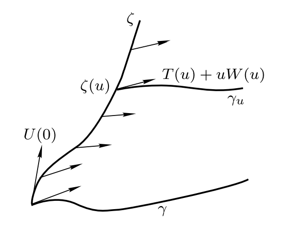
取$\gamma_u(t)=\exp_{\zeta(u)}t(T(u)+uW(u)),$
那么$\{\gamma_u\}$构成单参数测地线族, 且$\gamma_0\equiv \gamma.$
记其横截向量场限制在$\gamma$上为$U_1,$ 只需验证$U_1(0)=U(0),$
$\dot U_1(0)=\dot U(0).$ 一式由下式即得,
$$
U_1(0)=\left.\frac{\partial {} }{\partial {}u}\gamma_u(0)\right|_{u=0}=\dot\zeta(0)=U(0).
$$
对于二式, 记$\Gamma(t,u):=\gamma_u(t),$
$T_1:=d\Gamma\left(\frac{\partial {} }{\partial {}t}\right).$
回忆上节中的$[T,U]\equiv0,$ 类似地我们有:
$$
\dot U_1(0)=D_{\dot\gamma(0)}U_1=D_{U_1(0)}\dot\gamma=D_{\dot\zeta(0)}T_1.
$$
而我们知道, 由于$d\exp_O=\mathrm{id},$
$$
T_1(\zeta(u))=\left.\frac{\partial {} }{\partial {}t}\exp_{\zeta(u)}t(T(u)+uW(u))\right|_{t=0}=T(u)+uW(u).
$$
最后由于我们选取的是平行向量场, 就得到了
$$
\dot U_1(0)=D_{\dot\zeta(0)}(T(u)+uW(u))=W(0)=\dot U(0).
$$
引理 3. 设$U$是沿测地线$\gamma$的Jacobi场, 那么存在Jacobi场$U^\perp$满足$\left<{}U^\perp,\dot\gamma\right>,$ $a,b\in \mathbb{R},$ 使得
$$
U=U^\perp +(at+b)\dot\gamma.
$$
证: 首先我们可以看到,
$$
D_TD_T\left<{}U,\dot\gamma\right>=D_T\left<{}\dot U,\dot\gamma\right>=\left<{}\ddot U,\dot\gamma\right>=\left<{}-R_{\dot\gamma U}\dot\gamma,\dot\gamma\right>=-R(\dot\gamma,U,\dot\gamma,\dot\gamma)=0.
$$
因此$\left<{}U,\dot\gamma\right>(t)=a't+b'.$ 做正交化, 令
$$
a=\frac{a'}{|\dot\gamma|^2},\quad b=\frac{b'}{|\dot\gamma|^2},\quad U^\perp=U-(at+b)\dot\gamma,
$$
则$\left<{}U^\perp,\dot\gamma\right>=0,$ 且$U^\perp$的确是Jacobi场:
$$
\ddot{U}^\perp=\ddot U=-R_{\dot\gamma U}\dot\gamma=-R_{\dot\gamma U^\perp}\dot\gamma-(at+b)R_{\dot\gamma\dot\gamma}\dot\gamma=-R_{\dot\gamma U^\perp}\dot\gamma.
$$
因此垂直于$\dot\gamma$的Jacobi场是有意思的, 称其为正常Jacobi场.
由于$\left<{}U,\dot\gamma\right>=at+b,$
只要初值条件有$\left<{}U(0),\dot\gamma\right>=\left<{}\dot U(0),\dot\gamma\right>=0,$
那么$U(t)$就是正常Jacobi场. 类似地, 我们还有推论:
推论 4. 若$U$是沿测地线$\gamma$的Jacobi场, 存在$t_1\neq t_2,$ $\left<{}U,\dot\gamma\right>(t_1)=\left<{}U,\dot\gamma\right>(t_2)=0,$ 则$U$是正常Jacobi场.
现在我们用Jacobi场来了解$d\exp_x.$ 回忆第三章中,
我们得到了$d\exp_x$在半径方向总是不退化的. 现考虑$p\in M$处的奇异性,
取$X$为$p$点处切向量, 垂直于径向直线$t\mapsto tp.$ 取单参数测地线族:
$$
\gamma_u(t)=\exp_xt(T+uX),\quad T=p.
$$
由于$U(t)=d\exp_x tX,$
$U(0)=0,$ $\dot U(0)=X,$ $\left<{}X,T\right>=0,$
横截向量场$U$在基曲线$\gamma=\gamma_0$上的限制是正常Jacobi场.
由于$U(1)=d\exp_x X,$ 我们可以得到Gauss引理, 同时还有如下引理:
引理 5. $d\exp_x$在$p\in M_x$处退化的充要条件是$\gamma(t)=\exp_x tp$上存在不恒为零的正常Jacobi场, 在$x$与$\exp_xp$处取零.
若$d\exp_x$在$p\in M_x$处退化, 则称$p$是映射$\exp_x$的共轭点,
称$\exp_x p$为$x$沿测地线$\gamma(t)=\exp_x tp$的共轭点.
由刚刚的引理, 可以看出称之为”共轭”是有道理的: 这一关系具有对称性.
应用
接下来我们介绍第一个“整体性”定理, 即只需对流形全貌做一些拓扑,
几何假定后即可成立的性质.
定理 6 (Cartan-Hadamard定理). 设$M$是完备黎曼流形, 具非正截面曲率, 则$\,\forall\,x\in M,$ $\exp_x:M_x\rightarrow M$无共轭点; 当$M$是单连通完备黎曼流形时, 若$\exp_x:M_x\rightarrow M$无共轭点, 则$\exp_x$为微分同胚.
证: 只需证明对于任意测地线$\gamma,$ 其上非平凡正常Jacobi场$U,$
只要$U(0)=0,$ 则$\,\forall\,t>0,$ $U(t)\neq 0.$
定义$f(t)=\left<{}U,U\right>(t),$ 那么
$$
\ddot f=2\left(\left<{}\dot U,\dot U\right>+\left<{}\ddot U,U\right>\right)=2\left(\left<{}\dot U,\dot U\right>-\left<{}R_{\dot \gamma U}\dot\gamma,U\right>\right)\ge 0.
$$
最后一个不等号是因为$R(\dot\gamma,U,\dot\gamma,U)=K(\Pi)|\dot\gamma\wedge U|^2\le 0,$
$\Pi$为由$\left<{}\dot\gamma,U\right>$张成的子空间.
因此$f\ge 0$是凸函数, 结合Jacobi场的零点离散性就证明了结论.
事实上, 可以证明更精密的估计:
$$
\frac{d {}^2}{d {}t^2}|U(t)|\ge -|U(t)|\cdot |\dot\gamma(t)|\cdot|K(\Pi(t))|\ge 0.
$$
由该式可导出Rauch比较定理.
第二部分的证明只需说明$\exp_x$是覆盖映射. 由于底空间$M$是单连通的,
得到$\exp_x$是单射, 从而是微分同胚. 我们通过后面两个引理来说明这一点.
引理 7. 设$\varphi:M\rightarrow M'$是局部等距映射, $M$是完备的, 那么$\varphi$是覆盖映射, 且$M'$也是完备的.
证: 证明除了用到完备性与测地线性质外, 更多是拓扑上的技巧, 在此略过.
核心是利用等距变换保测地性,
说明局部上$\varphi=\exp_{\varphi(x)}\circ d\varphi \circ \exp_{x}^{-1}.$
引理 8. 设$M$是完备的黎曼流形, $x\in M,$ $\exp_x:M_x\rightarrow M$无共轭点, 则$\exp_x$是覆盖映射.
证: 取$g'=\exp_x^\ast g,$ 将$M$上的度量拉回到$M_x$上.
易见从原点出发的射线在$g'$意义下是$M_x$中的测地线, 那么由$M$的完备性,
这些射线均可无限延伸, 从而由Hopf-Rinow定理, $(M_x,g')$是完备的.
由$g'$定义, $\exp_x:(M_x,g')\rightarrow (M,g)$自然是局部等距映射,
那么由上述引理立即得到结论.
现在我们用Jacobi定理说明单连通空间形式的唯一性.
定理 9. 设$M,M'$是两个$n$维单连通的空间形式, 截面曲率为$c.$ 设$x\in M,$ $x'\in M',$ $\{e_i\},\{e'_i\}$分别是$M_x,M'_x$中的标准正交基. 那么存在唯一的等距映射$\varphi:M\rightarrow M',$ 使得$\varphi(x)=x',$ $d\varphi(e_i)=e'_i.$
证: 定理的证明较为繁琐, 在此省略. 证明不妨取$c=0,\pm 1,$
$M=S^n,\mathbb{R}^n,H^n$即可.
主要步骤是说明$\varphi=\exp_{x'}\circ\Phi\circ \exp_{x}^{-1}$即为所求.
其中$\Phi$是使得$\Phi(e_i)=e'_i$的唯一线性映照. 另外,
$c\le 0$时由Cartan-Hadamard定理可以直接取出这样的$\varphi,$
$c>0$时需要局部上取这样的$\varphi$再做合适的延拓.
证明中用到如下三个引理, 前两个引理用于展开Jacobi方程,
最后一个引理说明了等距变换的唯一性.
引理 10. 设$M$为$n$维空间形式, 截面曲率为$c.$ 设$x\in M,$ $\{e_i\}$为$M_x$标准正交基. 那么$M$的曲率张量满足:
$$
R_{e_ie_j}e_k=c(\delta_{ik}e_j-\delta_{jk}e_i),\quad 1\le i,j,k\le n.
$$
证: 只需证明依该式的确定义了一个曲率张量即可,
且该曲率张量的截面曲率也是$c.$ 那么由于截面曲率决定了曲率张量,
我们就建立了两个曲率张量的恒等关系.
推论 11. 记号同上一引理, 设$v$是$M_x$中单位向量, $v^\perp$是$v$的正交补, 那么
$$
R_{vw}v=
\left\{\begin{aligned}
&cw, &&w\in v^\perp,\\
&0, &&w=\alpha v.
\end{aligned}\right.
$$
引理 12. 设$\varphi_1,\varphi_2:M\rightarrow N$为两个局部等距, 满足$\,\exists\,x\in M,$ $\varphi_1(x)=\varphi_2(x)=y\in N,$ 且$d\varphi_1(x)=d\varphi_2(x):M_x\rightarrow M_y.$ 那么我们有$\varphi_1=\varphi_2.$
证: 取$M$中子集
$$
\mathscr{S}:=\{y\in M: \varphi_1(y)=\varphi_2(y),d\varphi_1(y)=d\varphi_2(y)\},
$$
说明其既开又闭即可(连通性假设总是默认的). 开集利用$\exp_y$说明,
闭集由连续性说明.
注意我们的主定理有值得注意的推论. 当$M=M'$时, 我们得到:
推论 13. 设$M$为$n$维完备单连通黎曼流形, 则$M$是空间形式当且仅当对于任意$x,x'\in M,$ $M_x,M_x'$中任意标准正交基$\{e_i\},\{e_i'\},$ 存在等距自变换$\varphi,$ 使得
$$
\varphi(x)=x', \quad d\varphi(e_i)=e_i'.
$$
这表明任一单连通空间形式必是齐性黎曼流形, 特别地$H^n$是齐性的,
而这并不能平凡地看出. 进一步可说明这些空间形式都是两点齐性的,
即对于任意$p_1,p_2,q_1,q_2\in M,$ $d(p_1,p_2)=d(q_1,q_2),$
存在等距映射$\varphi:M\rightarrow M,$ 使得$\varphi(p_i)=q_i,$ $i=1,2.$
推论 14. 所有单连通空间形式都是两点齐性的.
证: 由于流形是完备的,
存在测地线$\zeta,\xi$分别连接$p_1,p_2;q_1,q_2.$ 取等距变换$\varphi,$
使得$\varphi(\zeta(0))=\xi(0),$ $d\varphi(\dot\zeta(0))=\dot\xi(0).$
由等距变换保持测地线的性质即可知$\varphi(\zeta)=\xi,$ 命题得证.
文章最后更新于 2022-04-21 19:11:30
Jacobi field
Recall that if $\{\gamma_s\}$ is a single-parameter geodesic family, let $U$ be a transverse vector field.
Then $U$ is a Jacobi field restricted to the baseline $\gamma=\gamma_0$, satisfying the Jacobi equation:
$$
\ddot{U}+R_{\dot{\gamma}U}\dot{\gamma}=0.
$$
It is a system of second-order ordinary differential equations, so it has the following lemma:
Lemma 1. For any given geodesic $\gamma,$ $v,w\in M_{\gamma_0},$, there is a unique Jacobi field along $\gamma$, such that $U(0)=v,$ $\dot U(0)=w,$ and the zero points of the Jacobi field along the geodesic are discrete.
For the (unidirectional) lemma in the previous section, we have a more complete proposition:
Lemma 2. Given a geodesic $\gamma$ and a vector field $U,$ along it, it is a Jacobi field if and only if $U$ is a restriction on $\gamma$ of the transverse vector field of a certain single-parameter geodesic family $\{\gamma_s\}$, $\gamma_0\equiv \gamma.$
Certificate: It is only necessary to prove that $U$ is the case of Jacobi field.
Take the geodesic (or any curve) with $U(0)$ as the initial tangent vector $\zeta,$
Take the parallel vector field $T,W,$ on it to satisfy $T(0)=\dot\gamma(0),$ $W(0)=\dot U(0),$
We are going to knit a family of single-parameter geodesics.
Take $\gamma_u(t)=\exp_{\zeta(u)}t(T(u)+uW(u)),$
Then $\{\gamma_u\}$ forms a single-parameter geodesic family, and $\gamma_0\equiv \gamma.$
Note that its transverse vector field is limited to $\gamma$ as $U_1,$ and only need to verify $U_1(0)=U(0),$
$\dot U_1(0)=\dot U(0).$ One formula is obtained by the following formula,
$$
U_1(0)=\left.\frac{\partial {} }{\partial {}u}\gamma_u(0)\right|_{u=0}=\dot\zeta(0)=U(0).
$$
For the second formula, write $\Gamma(t,u):=\gamma_u(t),$
$T_1:=d\Gamma\left(\frac{\partial {} }{\partial {}t}\right).$
Recall $[T,U]\equiv0,$ from the previous section. Similarly we have:
$$
\dot U_1(0)=D_{\dot\gamma(0)}U_1=D_{U_1(0)}\dot\gamma=D_{\dot\zeta(0)}T_1.
$$
And we know that because $d\exp_O=\mathrm{id},$
$$
T_1(\zeta(u))=\left.\frac{\partial {} }{\partial {}t}\exp_{\zeta(u)}t(T(u)+uW(u))\right|_{t=0}=T(u)+uW(u).
$$
Finally, since we choose a parallel vector field, we get
$$
\dot U_1(0)=D_{\dot\zeta(0)}(T(u)+uW(u))=W(0)=\dot U(0).
$$
Lemma 3. Assume $U$ is the Jacobi field along the geodesic $\gamma$, then there is a Jacobi field $U^\perp$ that satisfies $\left<{}U^\perp,\dot\gamma\right>,$ $a,b\in \mathbb{R},$ such that
$$
U=U^\perp +(at+b)\dot\gamma.
$$
Certificate: First we can see,
$$
D_TD_T\left<{}U,\dot\gamma\right>=D_T\left<{}\dot U,\dot\gamma\right>=\left<{}\ddot U,\dot\gamma\right>=\left<{}-R_{\dot\gamma U}\dot\gamma,\dot\gamma\right>=-R(\dot\gamma,U,\dot\gamma,\dot\gamma)=0.
$$
Therefore, $\left<{}U,\dot\gamma\right>(t)=a't+b'.$ is orthogonalized, let
$$
a=\frac{a'}{|\dot\gamma|^2},\quad b=\frac{b'}{|\dot\gamma|^2},\quad U^\perp=U-(at+b)\dot\gamma,
$$
Then $\left<{}U^\perp,\dot\gamma\right>=0,$ and $U^\perp$ are indeed Jacobi fields:
$$
\ddot{U}^\perp=\ddot U=-R_{\dot\gamma U}\dot\gamma=-R_{\dot\gamma U^\perp}\dot\gamma-(at+b)R_{\dot\gamma\dot\gamma}\dot\gamma=-R_{\dot\gamma U^\perp}\dot\gamma.
$$
Therefore the Jacobi field perpendicular to $\dot\gamma$ is interesting and is called Normal Jacobi field.
Due to $\left<{}U,\dot\gamma\right>=at+b,$
As long as the initial value condition has $\left<{}U(0),\dot\gamma\right>=\left<{}\dot U(0),\dot\gamma\right>=0,$
Then $U(t)$ is the normal Jacobi field. Similarly, we also have the inference:
Corollary 4. If $U$ is the Jacobi field along the geodesic $\gamma$, and $t_1\neq t_2,$ $\left<{}U,\dot\gamma\right>(t_1)=\left<{}U,\dot\gamma\right>(t_2)=0,$ exists, then $U$ is the normal Jacobi field.
Now we use the Jacobi field to understand $d\exp_x.$. Recall from Chapter 3,
We have obtained that $d\exp_x$ is always non-degenerate in the radial direction. Now consider the singularity at $p\in M$,
Take $X$ as the tangent vector at point $p$, perpendicular to the radial straight line $t\mapsto tp.$ and take the single-parameter geodesic family:
$$
\gamma_u(t)=\exp_xt(T+uX),\quad T=p.
$$
Due to $U(t)=d\exp_x tX,$
$U(0)=0,$ $\dot U(0)=X,$ $\left<{}X,T\right>=0,$
The limit of the transverse vector field $U$ on the base curve $\gamma=\gamma_0$ is the normal Jacobi field.
Since $U(1)=d\exp_x X,$ we can get Gauss' Lemma, and also has the following lemma:
Lemma 5. The necessary and sufficient condition for $d\exp_x$ to degenerate at $p\in M_x$ is that there is a normal Jacobi field on $\gamma(t)=\exp_x tp$ that is not always zero, and it is zero at $x$ and $\exp_xp$.
If $d\exp_x$ degenerates at $p\in M_x$, then $p$ is said to be a map of $\exp_x$ conjugate point,
Call $\exp_x p$ as $x$ along the geodesic $\gamma(t)=\exp_x tp$ conjugate point.
From the lemma just mentioned, we can see that it makes sense to call it "conjugation": this relationship is symmetrical.
Application
Next we introduce the first one "wholeness" Theorem, that is, we only need to do some topology on the entire manifold,
Properties that can be established after geometric assumptions.
Theorem 6 (Cartan-Hadamard theorem). Assume $M$ is a complete Riemannian manifold with non-positive cross-section curvature, then $\,\forall\,x\in M,$ $\exp_x:M_x\rightarrow M$ has no conjugate points; when $M$ is a simply connected complete Riemannian manifold, if $\exp_x:M_x\rightarrow M$ has no conjugate points, then $\exp_x$ is a diffeomorphism.
Certificate: It is only necessary to prove that for any geodesic $\gamma,$ there is a non-trivial normal Jacobi field $U,$ on it
As long as $U(0)=0,$ then $\,\forall\,t>0,$ $U(t)\neq 0.$
Definition $f(t)=\left<{}U,U\right>(t),$ Then
$$
\ddot f=2\left(\left<{}\dot U,\dot U\right>+\left<{}\ddot U,U\right>\right)=2\left(\left<{}\dot U,\dot U\right>-\left<{}R_{\dot \gamma U}\dot\gamma,U\right>\right)\ge 0.
$$
The last inequality sign is because $R(\dot\gamma,U,\dot\gamma,U)=K(\Pi)|\dot\gamma\wedge U|^2\le 0,$
$\Pi$ is the subspace spanned by $\left<{}\dot\gamma,U\right>$.
Therefore $f\ge 0$ is a convex function, and the conclusion is proved by combining the zero-point discreteness of the Jacobi field.
In fact, a more precise estimate can be proved:
$$
\frac{d {}^2}{d {}t^2}|U(t)|\ge -|U(t)|\cdot |\dot\gamma(t)|\cdot|K(\Pi(t))|\ge 0.
$$
It can be derived from this formula Rauch's comparison theorem.
The second part of the proof only needs to show that $\exp_x$ is a covering map. Since the base space $M$ is simply connected,
Obtaining $\exp_x$ is an injection, and thus a diffeomorphism. We illustrate this point through the following two lemmas.
Lemma 7. Assume $\varphi:M\rightarrow M'$ is a local isometric map, $M$ is complete, then $\varphi$ is a covering map, and $M'$ is also complete.
Certificate: In addition to using completeness and geodesic properties, the proof is more about topological techniques, which will be skipped here.
The core is to use isometric transformation to ensure geodesic properties.
Explain locally $\varphi=\exp_{\varphi(x)}\circ d\varphi \circ \exp_{x}^{-1}.$
Lemma 8. Assume $M$ is a complete Riemannian manifold, $x\in M,$ $\exp_x:M_x\rightarrow M$ has no conjugate points, then $\exp_x$ is a covering map.
Certificate: Take $g'=\exp_x^\ast g,$ and pull the measure on $M$ back to $M_x$.
It is easy to see that the ray starting from the origin is the geodesic in $M_x$ in the sense of $g'$, then based on the completeness of $M$,
These rays can be extended infinitely, so the Hopf-Rinow theorem, $(M_x,g')$ is complete.
Defined by $g'$, $\exp_x:(M_x,g')\rightarrow (M,g)$ is naturally a local isometric mapping,
Then we get the conclusion immediately from the above lemma.
Now we use Jacobi's theorem to illustrate the uniqueness of the form of a simply connected space.
Theorem 9. Suppose $M,M'$ is the spatial form of two $n$-dimensional simply connected spaces, and the cross-sectional curvature is $c.$. Suppose $x\in M,$ $x'\in M',$ $\{e_i\},\{e'_i\}$ are the orthonormal bases in $M_x,M'_x$ respectively. Then there is a unique isometric mapping $\varphi:M\rightarrow M',$ such that $\varphi(x)=x',$ $d\varphi(e_i)=e'_i.$
Certificate: The proof of the theorem is relatively complicated and will be omitted here. The proof may as well take $c=0,\pm 1,$
$M=S^n,\mathbb{R}^n,H^n$ is enough.
The main step is to show that $\varphi=\exp_{x'}\circ\Phi\circ \exp_{x}^{-1}$ is what you want.
Among them, $\Phi$ is the only linear mapping that makes $\Phi(e_i)=e'_i$. In addition,
When $c\le 0$, the Cartan-Hadamard theorem can be used to directly extract $\varphi,$
When $c>0$ is used, it is necessary to take $\varphi$ locally and then make appropriate extensions.
The following three lemmas are used in the proof. The first two lemmas are used to expand the Jacobi equation,
The last lemma illustrates the uniqueness of isometric transformation.
Lemma 10. Let $M$ be the $n$-dimensional space form, and the cross-sectional curvature is $c.$. Let $x\in M,$ $\{e_i\}$ be the $M_x$ orthonormal basis. Then the curvature tensor of $M$ satisfies:
$$
R_{e_ie_j}e_k=c(\delta_{ik}e_j-\delta_{jk}e_i),\quad 1\le i,j,k\le n.
$$
Certificate: Just prove that a curvature tensor is indeed defined according to this formula,
And the cross-sectional curvature of this curvature tensor is also $c.$. Then since the cross-sectional curvature determines the curvature tensor,
We have established the identity relationship between the two curvature tensors.
Corollary 11. The notation is the same as the previous lemma, assuming $v$ is the unit vector in $M_x$, $v^\perp$ is the orthogonal complement of $v$, then
$$
R_{vw}v=
\left\{\begin{aligned}
&cw, &&w\in v^\perp,\\
&0, &&w=\alpha v.
\end{aligned}\right.
$$
Lemma 12. Let $\varphi_1,\varphi_2:M\rightarrow N$ be two local isometrics, satisfying $\,\exists\,x\in M,$ $\varphi_1(x)=\varphi_2(x)=y\in N,$ and $d\varphi_1(x)=d\varphi_2(x):M_x\rightarrow M_y.$, then we have $\varphi_1=\varphi_2.$
Certificate: Take the subset in $M$
$$
\mathscr{S}:=\{y\in M: \varphi_1(y)=\varphi_2(y),d\varphi_1(y)=d\varphi_2(y)\},
$$
Just show that it is both open and closed (the connectivity assumption is always the default). The open set is explained by $\exp_y$,
Closed sets are described by continuity.
Note that our main theorem has a noteworthy corollary. When $M=M'$, we get:
Corollary 13. Assume $M$ is a $n$-dimensional complete simply connected Riemannian manifold, then $M$ is a spatial form if and only if there is an isometric autotransformation $\varphi,$ for any orthonormal basis $\{e_i\},\{e_i'\},$ in any $x,x'\in M,$ $M_x,M_x'$ such that
$$
\varphi(x)=x', \quad d\varphi(e_i)=e_i'.
$$
This shows that any simply connected space form must be a homogeneous Riemannian manifold, especially $H^n$ is homogeneous,
And this cannot be seen trivially. It can be further explained that these spatial forms are all two-pointed,
That is, for any $p_1,p_2,q_1,q_2\in M,$ $d(p_1,p_2)=d(q_1,q_2),$
There is an isometric map $\varphi:M\rightarrow M,$ such that $\varphi(p_i)=q_i,$ $i=1,2.$
Corollary 14. All simply connected space forms are homogeneous at two points.
Certificate: Since the manifold is complete,
There are geodesics $\zeta,\xi$ connected to $p_1,p_2;q_1,q_2.$ respectively, and the isometric transformation $\varphi,$ is obtained.
makes $\varphi(\zeta(0))=\xi(0),$ $d\varphi(\dot\zeta(0))=\dot\xi(0).$
By maintaining the properties of the geodesic through isometric transformation, it can be seen that the proposition $\varphi(\zeta)=\xi,$ is proved.
The article was last updated on 2022-04-21 19:11:30